User documentation
SMOC (a.k.a MOC): Spatial coverages
Introduction to Space-MOCs
Space MOCs are an ensemble of HEALPix cells of mixed orders. They represent sky regions in an approximate way. They are designed for efficient calculations between sky regions.
The coordinates for Space-MOCs are always in IRCS at epoch J2000 by definition.
Space-MOCs can represent arbitrary shapes. Common examples are an approximated cone, an ensemble of approximated cones, or the coverage of a specific survey.
The following notebook is an introduction to manipulation of Space-MOCs with MOCPy:
As you saw, Space-MOCs can be visualized with either astropy+matplotlib or with the ipyaladin widget.
Space-MOC creation methods
Reading a MOC from a file or from a server
There are diverse ways to instantiate a MOC. A first approach is to get a MOC from a FITS file on our disk, or from a distant server that already has a pre-calculated MOC.
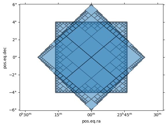
Calculating a MOC on the fly from a region of the sky
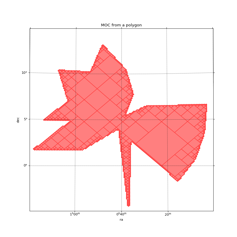
Here is a simple example of the creation of a MOC that fully covers a polygon defined by its vertices on the sky. The vertices are linked by great circles.
import astropy.units as u
import matplotlib.pyplot as plt
import numpy as np
from astropy.coordinates import Angle, SkyCoord
from mocpy import MOC, WCS

# The set of points delimiting the polygon in deg
vertices = np.array(
    [
        [18.36490956, 5.0],
        [15.7446692, 6.97214743],
        [16.80755056, 10.29852928],
        [13.36215502, 10.14616136],
        [12.05298691, 13.10706197],
        [9.54793022, 10.4556709],
        [8.7677627, 7.80921809],
        [9.71595962, 5.30855011],
        [7.32238541, 6.44905255],
        [0.807265, 6.53399616],
        [1.08855146, 3.51294225],
        [2.07615384, 0.7118289],
        [3.90690158, -1.61886929],
        [9.03727956, 2.80521847],
        [9.22274427, -4.38008174],
        [10.23563378, 4.06950324],
        [10.79931601, 3.77655576],
        [14.16533992, 1.7579858],
        [19.36243491, 1.78587203],
        [15.31732084, 5.0],
    ],
)
skycoord = SkyCoord(vertices, unit="deg", frame="icrs")
moc = MOC.from_polygon_skycoord(skycoord, complement=False, max_depth=9)

# Plot the MOC using matplotlib
fig = plt.figure(111, figsize=(10, 10))
# Define a astropy WCS easily
with WCS(
    fig,
    fov=20 * u.deg,
    center=SkyCoord(10, 5, unit="deg", frame="icrs"),
    coordsys="icrs",
    rotation=Angle(0, u.degree),
    # The gnomonic projection transforms great circles into straight lines.
    projection="TAN",
) as wcs:
    ax = fig.add_subplot(1, 1, 1, projection=wcs)
    # Call fill with a matplotlib axe and the `~astropy.wcs.WCS` wcs object.
    moc.fill(ax=ax, wcs=wcs, alpha=0.5, fill=True, color="red", linewidth=1)
    moc.border(ax=ax, wcs=wcs, alpha=1, color="red")

plt.xlabel("ra")
plt.ylabel("dec")
plt.title("MOC from a polygon")
plt.grid(color="black", linestyle="dotted")
plt.show()
(Source code, png, hires.png, pdf)

For a more extended description on how to create MOCs from diverse shapes, you can check the example notebooks Creating Space-MOCs from shapes and Creating MOCs out of astropy-regions..
Instantiating a MOC when we already know its HEALPix cells
This can be done with methods like from_string(),
from_healpix_cells(), from_depth29_ranges().
A simple MOC that represents the full sky is the MOC of order 0 that contains all the 12
HEALPix cells of the order 0. Creating it from a string looks like:
from mocpy import MOC

all_sky = MOC.from_str("0/0-11")  # the 12 cells of HEALPix at order 0
all_sky.display_preview()  # the inside of the MOC is represented in red with display_preview
(Source code, png, hires.png, pdf)

We could also take only odd numbered cells of order 1. Let’s use
from_json() that takes a dictionary:
from mocpy import MOC

moc = MOC.from_json({"1": [i for i in range(12 * 4) if i % 2 == 1]})
moc.display_preview()
(Source code, png, hires.png, pdf)

Useful methods
Calculating a Space-MOC sky area
This example shows how to calculate the sky area of a Space-MOC.
import astropy.units as u
import numpy as np
from mocpy import MOC

ALL_SKY = 4 * np.pi * u.steradian
moc = MOC.from_string("0/0-11")  # any other MOC instance will work
area = moc.sky_fraction * ALL_SKY
area = area.to(u.deg**2).value
Other examples (operations, use-cases)
Here are some other code examples manipulating MOC objects.
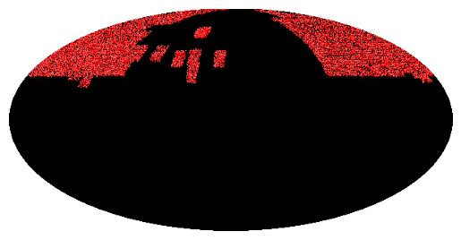
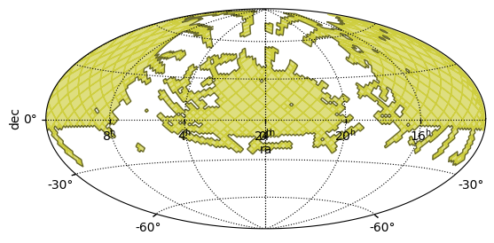
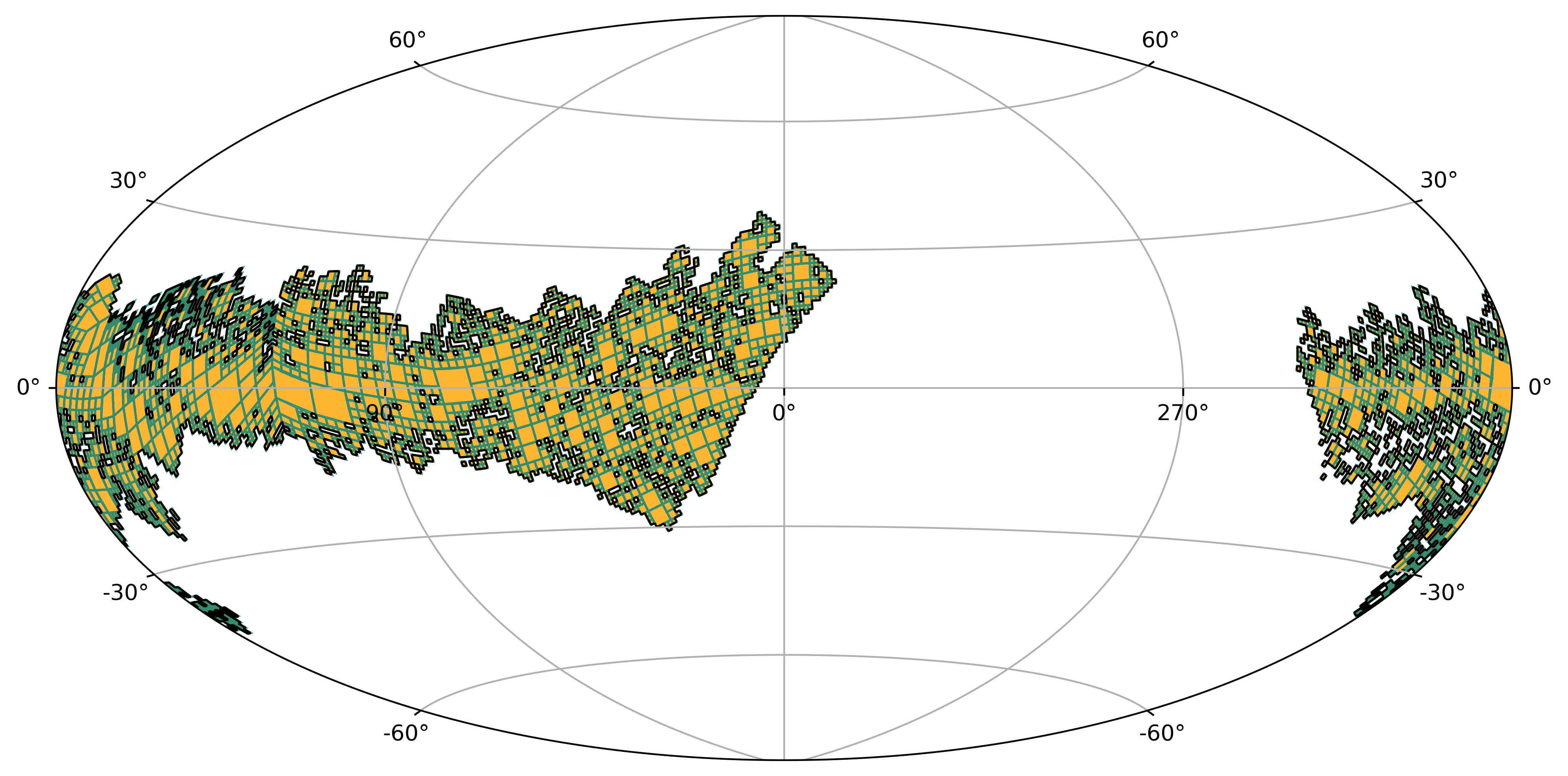
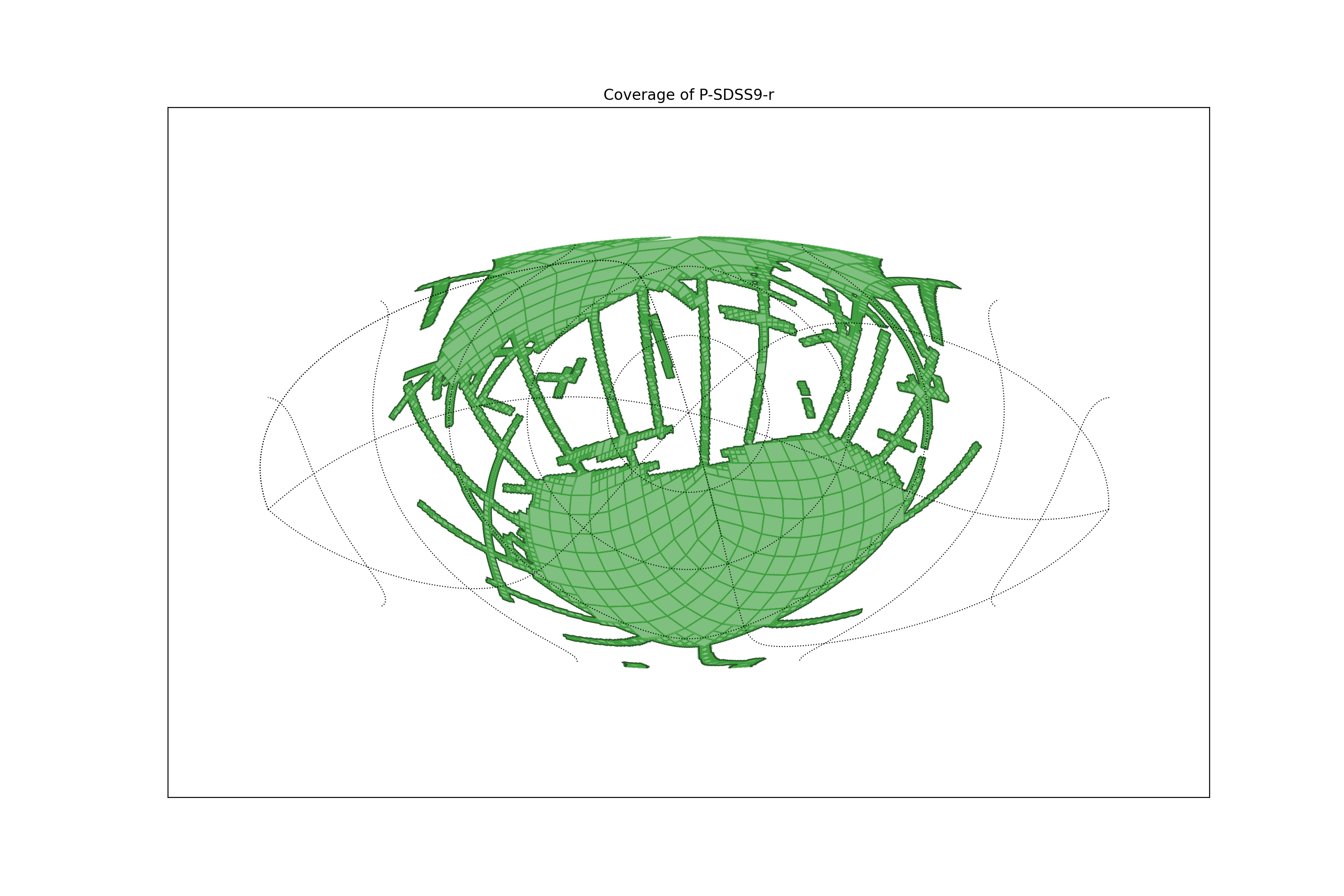
Loading and plotting the MOC of SDSS
This example:
Load the coverage of SDSS from a FITS file.
Plot the MOC by:
Defining a matplotlib figure.
Defining an astropy WCS representing the field of view of the plot.
Call the
fill()andborder()so that mocpy plot on a matplotlib axis.Set the axis labels, a title, enable the grid and plot the final figure.
import matplotlib.pyplot as plt
from astropy.visualization.wcsaxes.frame import EllipticalFrame
from astropy.wcs import WCS
from mocpy import MOC

# Load a MOC
filename = "./../../resources/P-SDSS9-r.fits"
moc = MOC.from_fits(filename)
# Plot the MOC using matplotlib
fig = plt.figure(111, figsize=(15, 10))
# Define a astropy WCS
wcs = WCS(
    {
        "naxis": 2,
        "naxis1": 1620,
        "naxis2": 810,
        "crpix1": 810.5,
        "crpix2": 405.5,
        "cdelt1": -0.2,
        "cdelt2": 0.2,
        "ctype1": "RA---AIT",
        "ctype2": "DEC--AIT",
    },
)
ax = fig.add_subplot(1, 1, 1, projection=wcs, frame_class=EllipticalFrame)
# Call fill with a matplotlib axe and the `~astropy.wcs.WCS` wcs object.
moc.fill(ax=ax, wcs=wcs, alpha=0.5, fill=True, color="green")
moc.border(ax=ax, wcs=wcs, alpha=0.5, color="black")
ax.set_aspect(1.0)
plt.xlabel("ra")
plt.ylabel("dec")
plt.title("Coverage of P-SDSS9-r")
plt.grid(color="black", linestyle="dotted")
plt.show()
(Source code, png, hires.png, pdf)

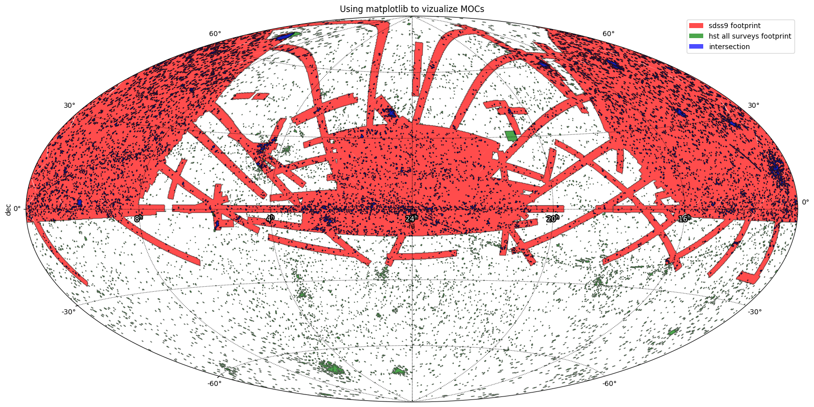
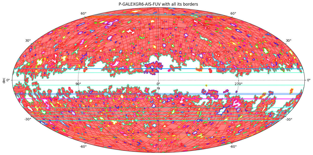
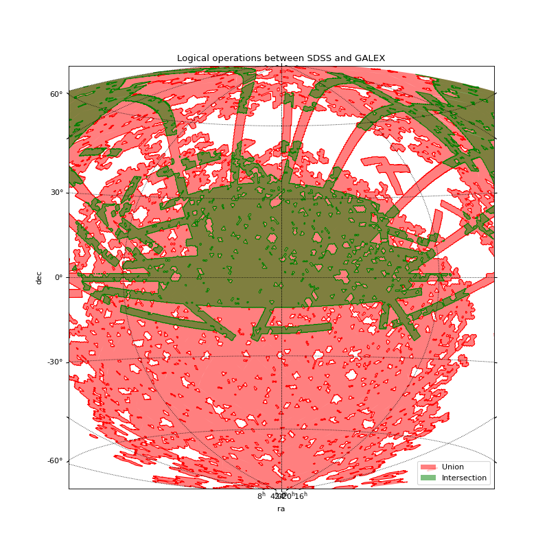
Intersection between GALEX and SDSS
This example:
Load the coverages of SDSS and GALEX from FITS files.
Compute their intersection
Compute their union
Plot the resulting intersection and union on a same matplotlib axis.
import matplotlib.pyplot as plt
from astropy.visualization.wcsaxes.frame import EllipticalFrame
from astropy.wcs import WCS
from mocpy import MOC

# Load Galex and SDSS
sdss = MOC.from_fits("./../../resources/P-SDSS9-r.fits")
galex = MOC.from_fits("./../../resources/P-GALEXGR6-AIS-FUV.fits")
# Compute their intersection
inter = sdss & galex
union = sdss + galex
# Plot the MOC using matplotlib
fig = plt.figure(111, figsize=(10, 8))
# Define a astropy WCS
wcs = WCS(
    {
        "naxis": 2,
        "naxis1": 3240,
        "naxis2": 1620,
        "crpix1": 1620.5,
        "crpix2": 810.5,
        "cdelt1": -0.1,
        "cdelt2": 0.1,
        "ctype1": "RA---AIT",
        "ctype2": "DEC--AIT",
    },
)
ax = fig.add_subplot(1, 1, 1, projection=wcs, frame_class=EllipticalFrame)
# Call fill with a matplotlib axe and the `~astropy.wcs.WCS` wcs object.
union.fill(
    ax=ax,
    wcs=wcs,
    alpha=0.5,
    fill=True,
    color="blue",
    linewidth=0,
    label="Union",
)
union.border(ax=ax, wcs=wcs, alpha=1, color="black")

inter.fill(
    ax=ax,
    wcs=wcs,
    alpha=0.5,
    fill=True,
    color="green",
    linewidth=0,
    label="Intersection",
)
inter.border(ax=ax, wcs=wcs, alpha=1, color="black")
ax.legend()
ax.set_aspect(1.0)
plt.xlabel("ra")
plt.ylabel("dec")
plt.title("Logical operations between SDSS and GALEX")
plt.grid(color="black", linestyle="dotted")
plt.show()
(Source code, png, hires.png, pdf)
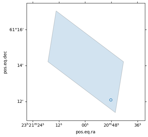
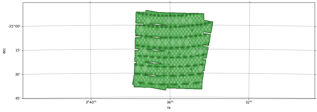
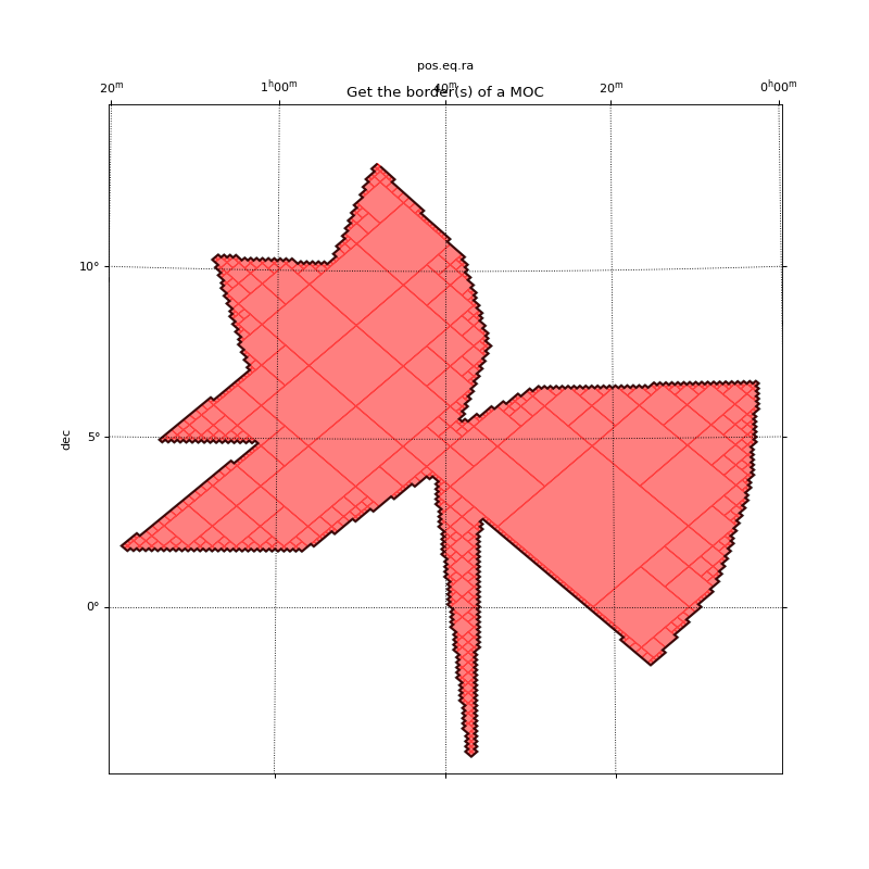
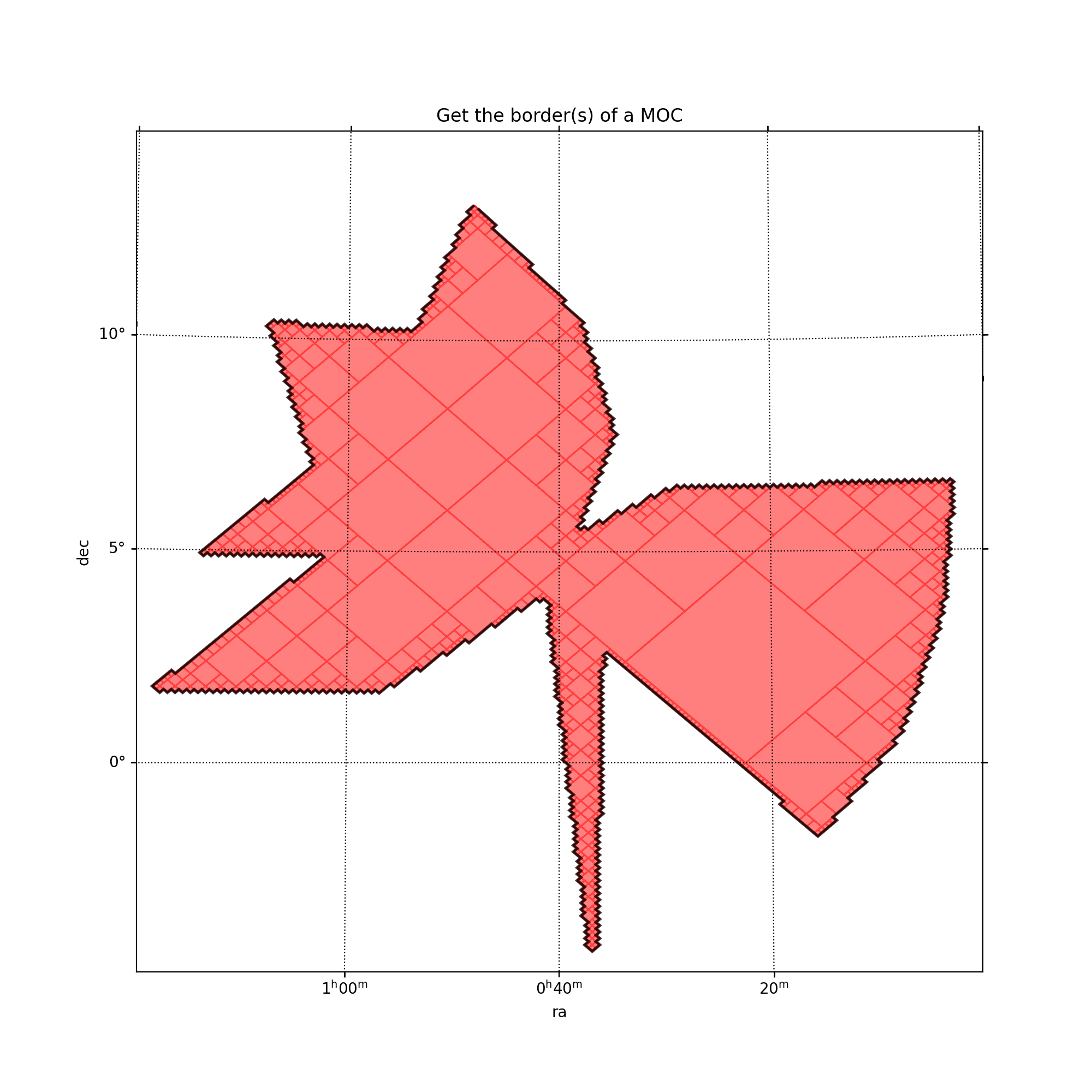
Get the border(s) of a MOC
This example shows how to call get_boundaries. The borders are returned as a list of SkyCoord each defining one border.
In this example:
The sky coordinates defining the border of the MOC are projected to the pixel image system.
Then, a matplotlib path is defined from the projected vertices.
Finally the path is plot on top of the MOC.
import astropy.units as u
import matplotlib.pyplot as plt
import numpy as np
from astropy.coordinates import Angle, SkyCoord
from matplotlib.patches import PathPatch
from matplotlib.path import Path
from mocpy import MOC, WCS

moc = MOC.from_fits("polygon_moc.fits")
skycoords = moc.get_boundaries()

# Plot the MOC using matplotlib
fig = plt.figure(111, figsize=(10, 10))
# Define a astropy WCS easily
with WCS(
    fig,
    fov=20 * u.deg,
    center=SkyCoord(10, 5, unit="deg", frame="icrs"),
    coordsys="icrs",
    rotation=Angle(0, u.degree),
    # The gnomonic projection transforms great circles into straight lines.
    projection="TAN",
) as wcs:
    ax = fig.add_subplot(1, 1, 1, projection=wcs)
    # Call fill with a matplotlib axe and the `~astropy.wcs.WCS` wcs object.
    moc.fill(ax=ax, wcs=wcs, alpha=0.5, fill=True, color="red", linewidth=1)
    moc.border(ax=ax, wcs=wcs, alpha=1, color="red")

    # Plot the border
    from astropy.wcs.utils import skycoord_to_pixel

    x, y = skycoord_to_pixel(skycoords[0], wcs)
    p = Path(np.vstack((x, y)).T)
    patch = PathPatch(p, color="black", fill=False, alpha=0.75, lw=2)
    ax.add_patch(patch)

plt.xlabel("ra")
plt.ylabel("dec")
plt.title("Get the border(s) of a MOC")
plt.grid(color="black", linestyle="dotted")
plt.show()
(Source code, png, hires.png, pdf)
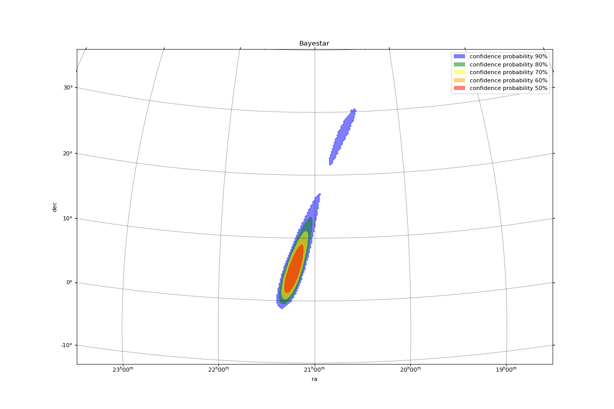
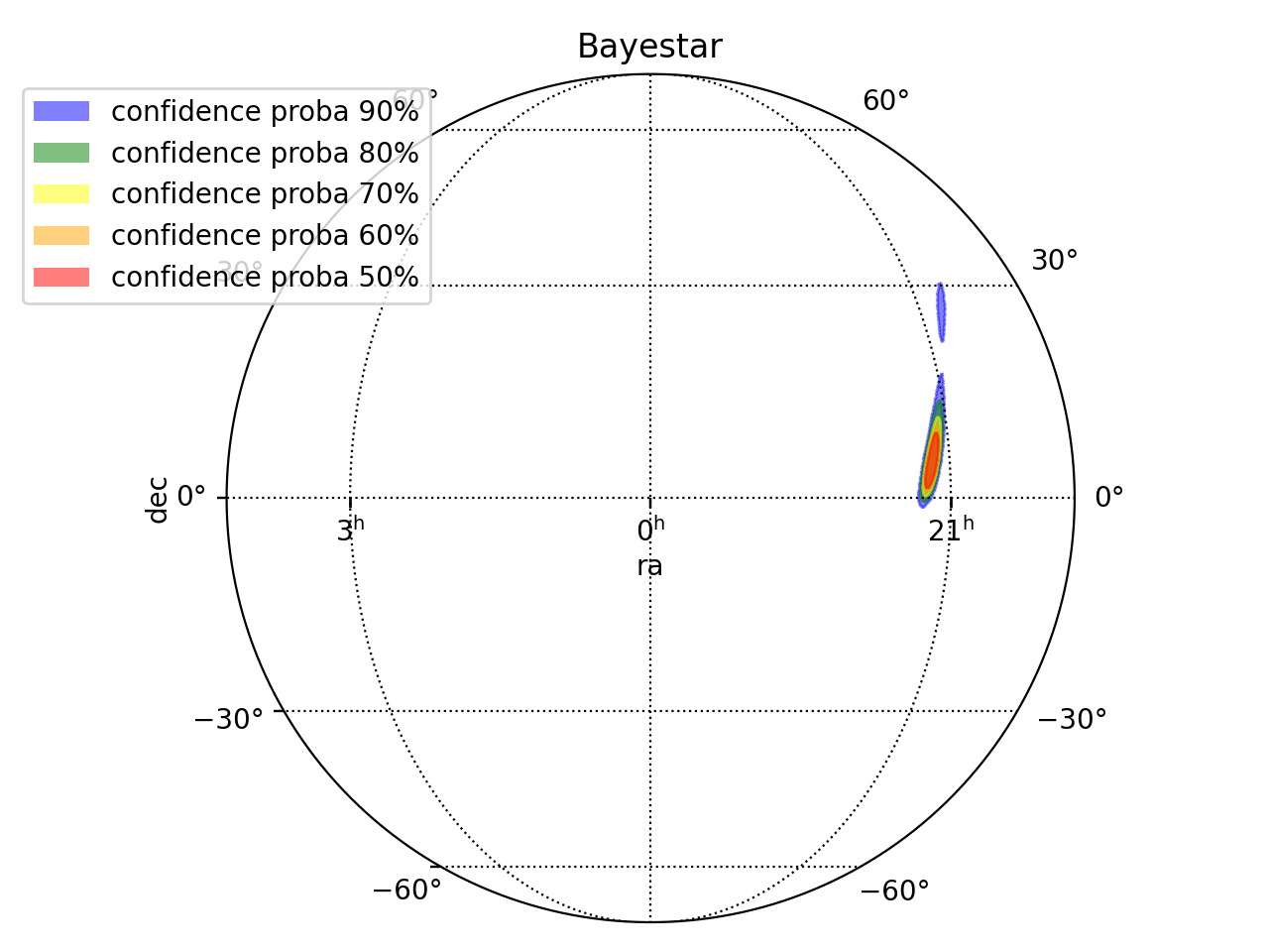
Gravitational Waves MOCs
This example shows the probability confidence regions of gravitational waves. HEALPix cells are given under the uniq pixel notation. Each pixel is associated with a specific probability density value. We convert this into a probability by multiplying it with the area of each cell. Then, we can create a MOC from which a GW has x% of chance of being localized in it. By definition the MOC which has 100% of chance of containing a GW is the full sky MOC.
import astropy.units as u
import matplotlib.pyplot as plt
import numpy as np
from astropy.io import fits
from astropy.visualization.wcsaxes.frame import EllipticalFrame
from astropy.wcs import WCS
from mocpy import MOC

# this can be found in mocpy's repository
# https://github.com/cds-astro/mocpy/blob/master/resources/bayestar.multiorder.fits
fits_image_filename = "./../../resources/bayestar.multiorder.fits"

with fits.open(fits_image_filename) as hdul:
    hdul.info()
    data = hdul[1].data
    max_order = hdul[1].header["MOCORDER"]

uniq = data["UNIQ"]
probdensity = data["PROBDENSITY"]

# let's convert the probability density into a probability
orders = (np.log2(uniq // 4)) // 2
area = 4 * np.pi / np.array([MOC.n_cells(int(order)) for order in orders]) * u.sr
prob = probdensity * area

# now we create the mocs corresponding to different probability thresholds
cumul_to = np.linspace(0.5, 0.9, 5)[::-1]
colors = ["blue", "green", "yellow", "orange", "red"]
mocs = [
    MOC.from_valued_healpix_cells(uniq, prob, max_order, cumul_to=c) for c in cumul_to
]


# Plot the MOC using matplotlib
fig = plt.figure(111)
# Define a astropy WCS
wcs = WCS(
    {
        "naxis": 2,
        "naxis1": 3240,
        "naxis2": 3240,
        "crpix1": 1620.5,
        "crpix2": 1620.5,
        "cdelt1": -0.0353,
        "cdelt2": 0.0353,
        "ctype1": "RA---SIN",
        "ctype2": "DEC--SIN",
    },
)

ax = fig.add_subplot(1, 1, 1, projection=wcs, frame_class=EllipticalFrame)
# Call fill with a matplotlib axe and the `~astropy.wcs.WCS` wcs object.
for moc, c, col in zip(mocs, cumul_to, colors):
    moc.fill(
        ax=ax,
        wcs=wcs,
        alpha=0.5,
        linewidth=0,
        fill=True,
        color=col,
        label="confidence proba " + str(round(c * 100)) + "%",
    )
    moc.border(ax=ax, wcs=wcs, alpha=0.5, color=col)
ax.legend(loc="upper center", bbox_to_anchor=(0, 1))
ax.set_aspect(1.0)
plt.xlabel("ra")
plt.ylabel("dec")
plt.title("Bayestar")
plt.grid(color="black", linestyle="dotted")
plt.tight_layout()
plt.show()
(Source code, png, hires.png, pdf)
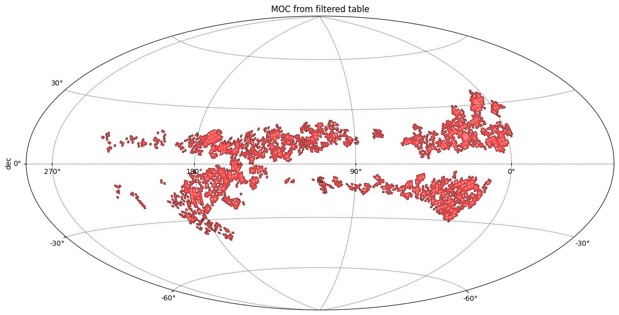
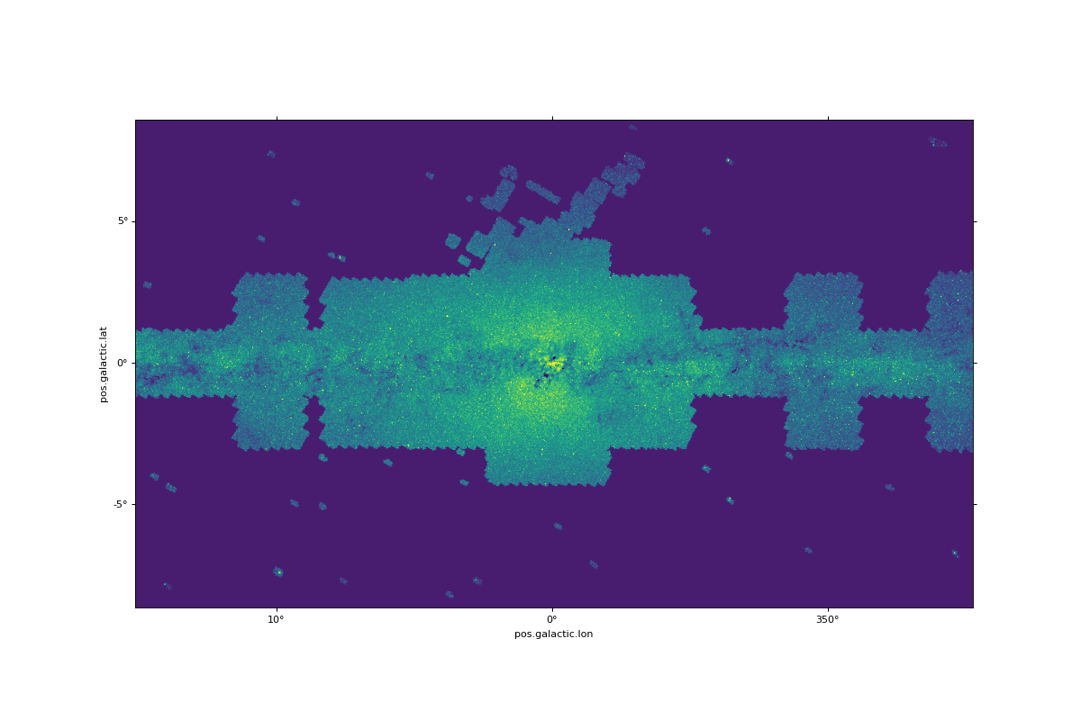
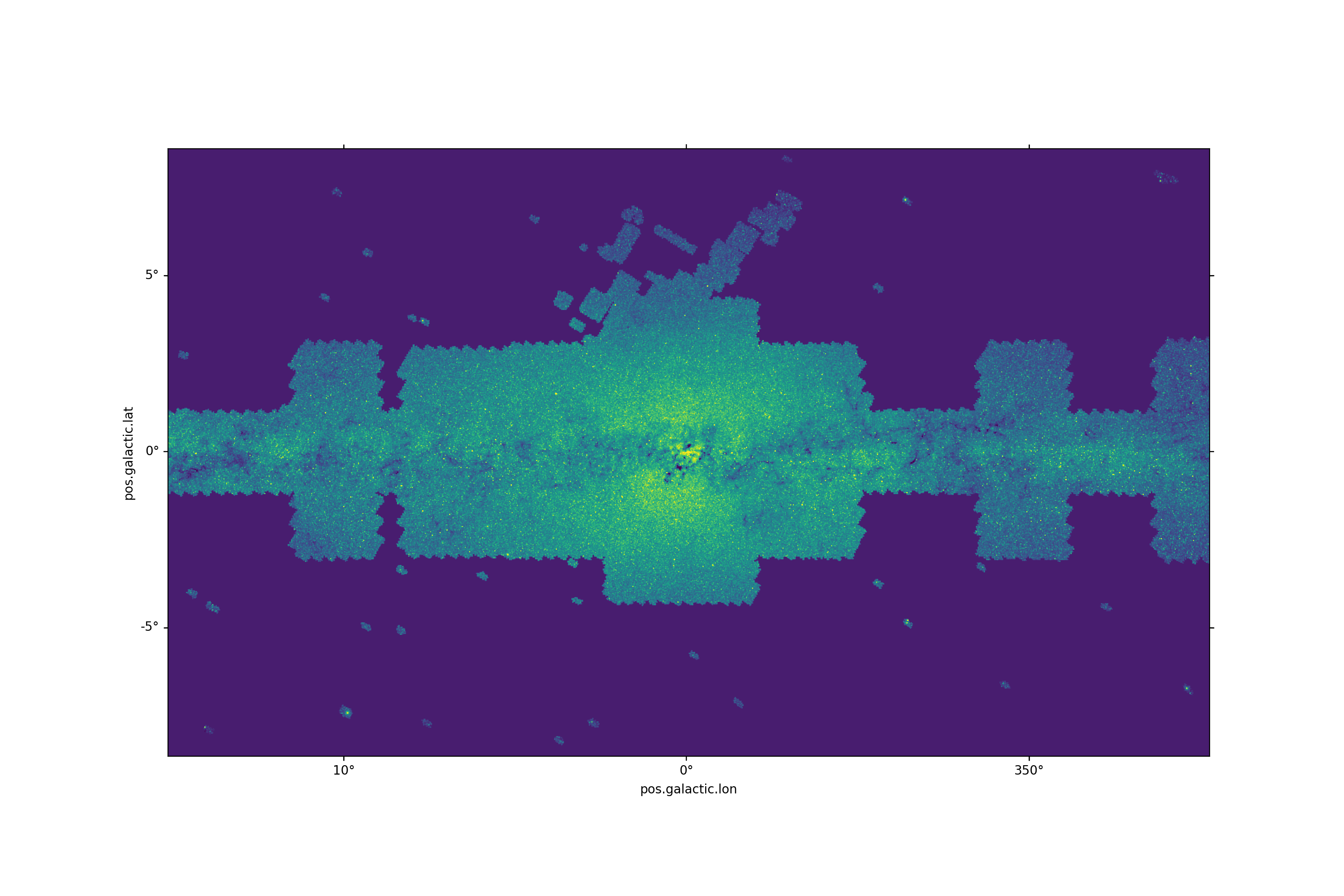
Performing computation on the pixels of an FITS image lying in a MOC
This example shows how a MOC can filter pixels from a specific FITS image (i.e. associated with a WCS). These pixels can then be retrieved from the image for performing some computations on them: e.g. mean, variance analysis thanks to numpy/scikit-learn…
import astropy.units as u
import matplotlib.pyplot as plt
import numpy as np
from astropy.io import fits
from astropy.visualization import simple_norm
from astropy.wcs import WCS as WCS
from mocpy import MOC

# load 2MASS cutout covering the galactic plane
hdu = fits.open(
    "http://alasky.u-strasbg.fr/hips-image-services/hips2fits?hips=CDS%2FP%2F2MASS%2FK&width=1200&height=700&fov=30&projection=TAN&coordsys=galactic&rotation_angle=0.0&object=gal%20center&format=fits",
)

# load Spitzer MOC
moc = MOC.from_fits("http://skies.esac.esa.int/Spitzer/IRAC1_bright_ISM/Moc.fits")

# create WCS from 2MASS image header
twomass_wcs = WCS(header=hdu[0].header)

# compute skycoords for every pixel of the image
width = hdu[0].header["NAXIS1"]
height = hdu[0].header["NAXIS2"]

xv, yv = np.meshgrid(np.arange(0, width), np.arange(0, height))
skycoords = twomass_wcs.pixel_to_world(xv, yv)

ra, dec = skycoords.icrs.ra.deg, skycoords.icrs.dec.deg
# Get the skycoord lying in the MOC mask
mask_in_moc = moc.contains(ra * u.deg, dec * u.deg)

img = hdu[0].data
img_test = img.copy()

# Set to zero the pixels that do not belong to the MOC
img_test[~mask_in_moc] = 0

# Plot the filtered pixels image
fig = plt.figure(111, figsize=(15, 10))
ax = fig.add_subplot(1, 1, 1, projection=twomass_wcs)

im = ax.imshow(
    img_test,
    origin="lower",
    norm=simple_norm(hdu[0].data, "sqrt", vmin=-1, vmax=150),
)
plt.show()
(Source code, png, hires.png, pdf)
# Sum of pixels lying in the MOC
np.sum(img[mask_in_moc])

# Sum of pixels of the whole image
np.sum(img)
TMOC: Temporal coverages
The TimeMOC class represents a temporal coverage.
Please check the following notebooks if you want to know more about time MOCs.
STMOC: Space & Time coverages
Space-Time coverages are a new feature of mocpy since its version 0.7.0 and are bind spatial and temporal coverages together.
The standard description is published by the IVOA here.
Space-Time coverages allow to:
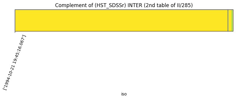
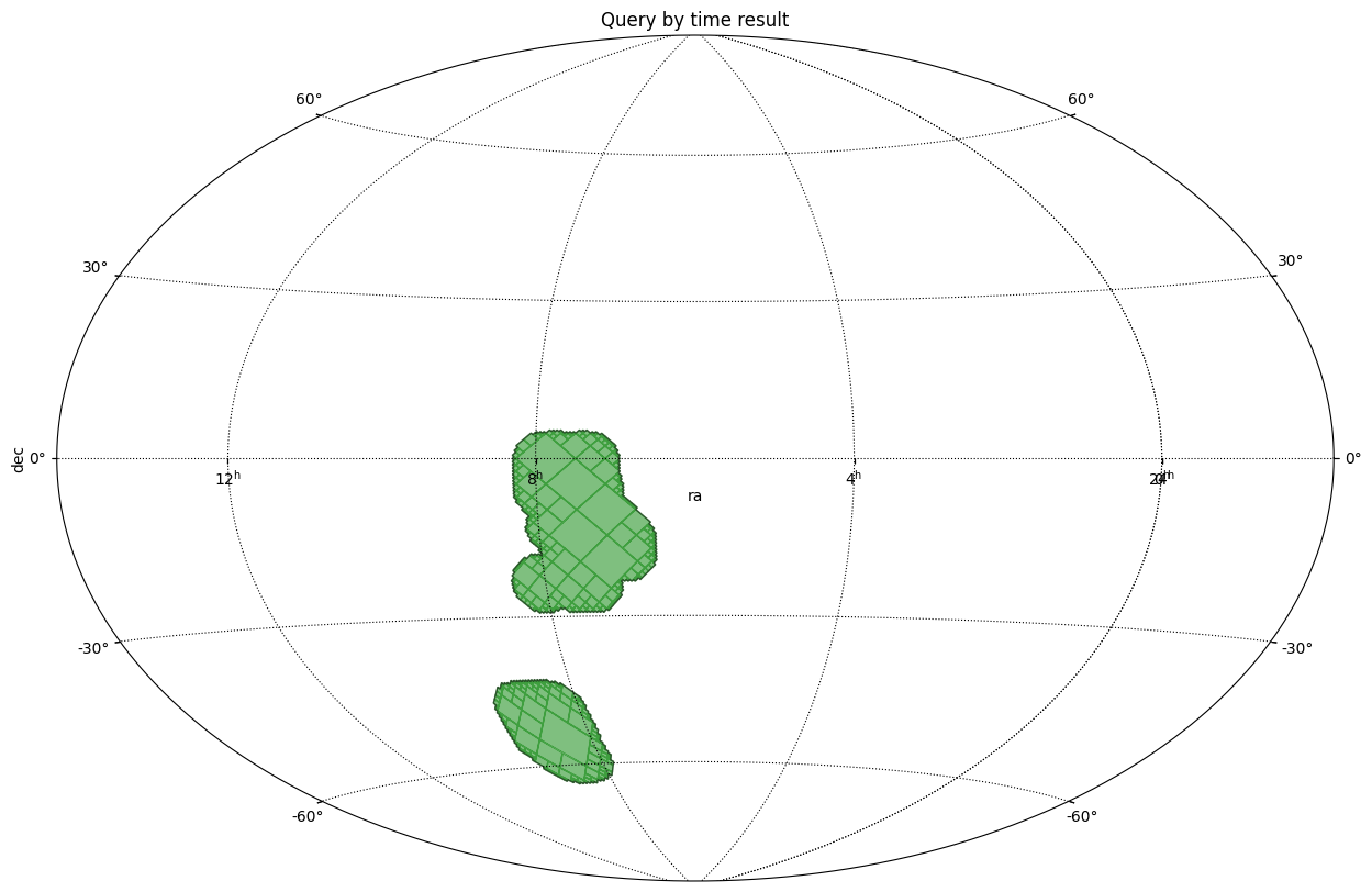
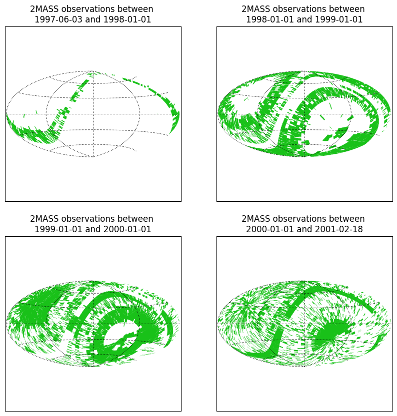
Retrieve the spatial coverage observed by a mission within a set of time frames (i.e.
astropy.time.Timeranges).Retrieve the temporal coverage observed by a mission within a spatial coverage.
As we do for spatial or temporal coverages, one can also perform the union, intersection or difference between two Space-Time coverages.
Please check the following notebooks if you want to know more about space-time MOCs.
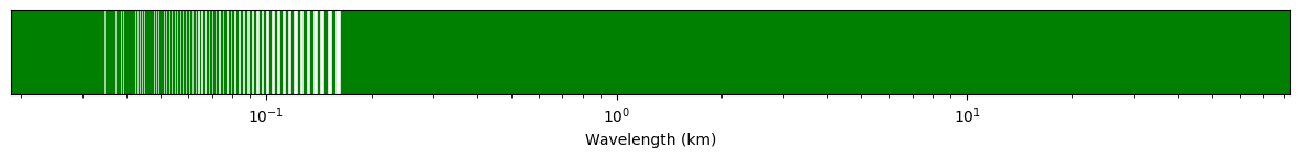
FMOC: Frequency coverages
Please check the following notebooks if you want to know more about frequency MOCs.
SFMOC: Space-Frequency coverages
Creating SF-MOC instances
1. From a FITS, ASCII, JSON file
The SFMOC class allows manipulation and generation of
Space-Frequency Multi-Order Coverages (SF-MOCs).
New empty SF-MOC new_empty:
>>> from mocpy import SFMOC
>>> SFMOC.new_empty(max_order_frequency=40, max_order_space=12)
f40/ s12/
Loading an SF-MOC from a FITS, JSON or ASCII file load:
>>> # we generate a fake ASCII file
>>> from tempfile import NamedTemporaryFile
>>> with NamedTemporaryFile(delete_on_close=False) as tf:
...     tf.write(b"f20/0-100 s12/0-100")
...     tf.close()
...     # and we read it
...     SFMOC.load(tf.name, format="ascii")
19
f14/0
15/2
18/24
20/100
s9/0
10/4-5
11/24
12/100
f20/ s12/
This illustrated the load method that we use when we have a MOC in a file, but for
ASCII strings, one can also directly use from_string:
>>> SFMOC.from_string("f15/2 s12/1")
f15/2
s12/1
f15/ s12/
Creating SF-MOCs from physical parameters:
2. From frequency-position “points”
In from_frequencies_and_positions, we give a set of frequency-position
“points” and the SF-MOC will be built from the cells containing these punctual data at
the maximum requested order. Use the utility functions
spatial_resolution_to_order to chose the space resolution and
relative_precision_to_order to chose the frequency resolution.
>>> import astropy.units as u
>>> from mocpy import SFMOC
>>> SFMOC.from_frequencies_and_positions(
...     [0.01, 0.1, 1, 10, 100] * u.Hz,
...     lon=[0, 1, 2, 3, 4] * u.deg, lat=[0, 1, 2, 3, 4] * u.deg,
...     max_order_frequency=25, max_order_space=8)
f25/19173961
s8/311296
f25/20372333
s8/311316
f25/21570706
s8/311378
f25/22769078
s8/311558
f25/23967451
s8/311624
f25/ s8/
3. From frequency ranges associated to punctual positions
With mocpy.SFMOC.from_frequency_ranges_and_positions we do not get a single cell in
frequency, bu the cells covering a given frequency band/range:
>>> import astropy.units as u
>>> from mocpy import SFMOC
>>> SFMOC.from_frequency_ranges_and_positions(
...     frequencies_min=[0.01, 0.1, 1, 10, 100] * u.Hz,
...     frequencies_max=[0.1, 1, 10, 100, 1000] * u.Hz,
...     lon=[0, 1, 2, 3, 4] * u.deg, lat=[0, 1, 2, 3, 4] * u.deg,
...     max_order_frequency=6, max_order_space=8)
f5/18
6/
s8/311296
f6/38
s8/311296 311316
f6/39-40
s8/311316
f6/41
s8/311316 311378
f6/42
s8/311378
f6/43
s8/311378 311558
f6/44
s8/311558
f6/45
s8/311558 311624
f5/23
6/
s8/311624
f6/ s8/
4. From frequency ranges associated to Space-MOCs
In from_spatial_coverages, the positions are not punctual anymore. They
are represented by S-MOCs, which can be built with the MOC module. Let’s for
example build an SF-MOC from a square observation in two given frequency bands:
>>> from mocpy import MOC, SFMOC
>>> import astropy.units as u
>>> # a MOC representing a field of view
>>> moc = MOC.from_box(lon=0*u.deg, lat=0*u.deg, a=2*u.deg, b=2*u.deg,
...                    angle=0*u.deg, max_depth=10)
>>> # we use the same moc twice, and give two ranges
>>> sfmoc_fov = SFMOC.from_spatial_coverages(
...    frequencies_min=([200, 300]*u.nm).to(u.Hz, equivalencies=u.spectral()),
...    frequencies_max=([100, 200]*u.nm).to(u.Hz, equivalencies=u.spectral()),
...    spatial_coverages=[moc, moc],
...    max_order_frequency=13)
Utilities
To inspect an SFMOC instance, one can read its max_order,
min_frequency and max_frequency properties. We can also
check wether it is empty with is_empty. Let’s use sfmoc_fov from the
previous example:
>>> sfmoc_fov.max_order
(13, 10)
>>> sfmoc_fov.is_empty()
False
>>> sfmoc_fov.min_frequency
<Quantity 9.93276847e+14 Hz>
>>> sfmoc_fov.max_frequency
<Quantity 3.01303312e+15 Hz>
General manipulation
Check wether a list of “punctual” position/frequency values fall within an SF-MOC:
>>> from mocpy import SFMOC, MOC
>>> import astropy.units as u
>>> # we generate an SF-MOC from a cone and a range of frequencies
>>> moc = MOC.from_cone(0*u.deg, 0*u.deg, radius=10*u.deg, max_depth=10)
>>> sfmoc_cone = SFMOC.from_spatial_coverages(0.01*u.Hz, 100*u.Hz,
...                                           moc, max_order_frequency=40)
>>> # one inside, one outside
>>> sfmoc_cone.contains([10, 10000]*u.Hz, [0.1, 20]*u.deg, [0.1, 20]*u.deg)
array([ True, False])
Fold operation on one of the SF-MOC dimensions, use mocpy.SFMOC.query_by_frequency or
query_by_space
>>> from mocpy import FrequencyMOC as FMOC
>>> fmoc = FMOC.from_frequency_ranges(15, 0.1*u.Hz, 1*u.Hz)
>>> moc = sfmoc_cone.query_by_frequency(fmoc)
>>> type(moc)
<class 'mocpy.moc.moc.MOC'>
Here we recover the Space-MOC corresponding to the parts of the sfmoc_cone coverage
with frequencies within fmoc.