First steps with Frequency MOCs

# Standard Library
from pathlib import Path

import matplotlib.pyplot as plt

# General and astronomy packages
import numpy as np
from astropy.units import Unit
from maser.data import Data

# Specific to FMOCs
from mocpy import FrequencyMOC

We use a file from the Cassini/RPWS/HFR database. This radio instrument has a configurable spectral sampling. The data file is a level 2 data file, containing the centers and widths of each spectral bin.

The file (and many others) is available for download here: https://lesia.obspm.fr/kronos/data/2012_091_180/n2/

file = Path("../resources/FMOC/P2012180.20")

We load the data using the maser.data module, which recognizes the file

n2 = Data(file)
n2.fields

dict_keys(['ydh', 'num', 't97', 'f', 'dt', 'df', 'autoX', 'autoZ', 'crossR', 'crossI', 'ant'])

n2.dataset

'co_rpws_hfr_kronos_n2'

Spectral sweeps are available as a generator using the .sweeps property.

sweep = next(n2.sweeps)
print(f"This sweep has {len(sweep.data)} spectral steps")
sweep.data.dtype

This sweep has 359 spectral steps

dtype([('ydh', '<u4'), ('num', '<u4'), ('t97', '<f8'), ('f', '<f4'), ('dt', '<f4'), ('df', '<f4'), ('autoX', '<f4'), ('autoZ', '<f4'), ('crossR', '<f4'), ('crossI', '<f4'), ('ant', 'i1')])

Then we get the central frequency and widths for each channel and we can infer the minimumm and maximum frequencyes for each sweep.

# Central frequency
freqs = np.float64(sweep.data["f"]) * Unit("kHz")
# Width of each channel
dfreq = np.float64(sweep.data["df"]) * Unit("kHz")

fmin = freqs - dfreq / 2
fmax = freqs + dfreq / 2

fmin

$[3.59346,~3.7664249,~3.9476776,~\dots,~15812.5,~15912.5,~16012.5] \; \mathrm{kHz}$

fmax

$[3.77774,~3.9595749,~4.1501226,~\dots,~15837.5,~15937.5,~16037.5] \; \mathrm{kHz}$

Now let’s start playing with this F-MOCs.

fmoc = FrequencyMOC.from_frequency_ranges(order=50, min_freq=fmin, max_freq=fmax)

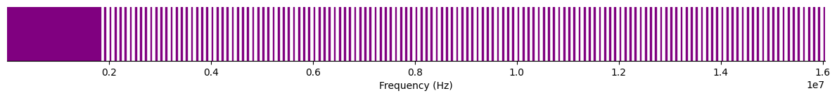
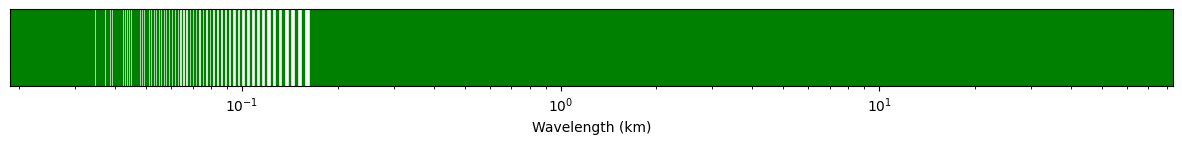
We can plot it in frequency or wavelength

fig, ax = plt.subplots(figsize=(15, 1))
fmoc.plot_frequencies(ax, color="purple")
# this method plots the frequency ranges in log scale by default
# but we can change it to linear if needed
ax.set(xscale="linear")
# and any customization on the ax of fig objects will work too
ax.spines[["left", "top", "right"]].set_visible(False)

fig, ax = plt.subplots(figsize=(15, 1))
fmoc.plot_wavelengths(ax, color="g", length_unit="km")

We create a dictionnary of FMOCs with less and less precise order ranging from 50 to 10.

print(
    f"we first create an initial FMOC at order {fmoc.max_order}"
    " and then generate the dictionnary",
)
fmocs = {n: fmoc.degrade_to_order(n) for n in np.linspace(50, 10, 5, dtype=int)}

we first create an initial FMOC at order 50 and then generate the dictionnary

for order in fmocs:
    print(
        f"At order {order}, this F-MOC has {len(fmocs[order].to_hz_ranges())} "
        "non overlapping spectral intervals",
    )

At order 50, this F-MOC has 143 non overlapping spectral intervals
At order 40, this F-MOC has 143 non overlapping spectral intervals
At order 30, this F-MOC has 143 non overlapping spectral intervals
At order 20, this F-MOC has 143 non overlapping spectral intervals
At order 10, this F-MOC has 1 non overlapping spectral intervals

for order in fmocs:
    print(
        f"At order {order}, the spectrum covers {round(fmocs[order].to_hz_ranges()[0][0])} Hz"
        " to {round(fmocs[order].to_hz_ranges()[-1][1])} Hz",
    )

At order 50, the spectrum covers 3593 Hz to {round(fmocs[order].to_hz_ranges()[-1][1])} Hz
At order 40, the spectrum covers 3593 Hz to {round(fmocs[order].to_hz_ranges()[-1][1])} Hz
At order 30, the spectrum covers 3593 Hz to {round(fmocs[order].to_hz_ranges()[-1][1])} Hz
At order 20, the spectrum covers 3593 Hz to {round(fmocs[order].to_hz_ranges()[-1][1])} Hz
At order 10, the spectrum covers 3584 Hz to {round(fmocs[order].to_hz_ranges()[-1][1])} Hz

Next step is FT-MOC, in order to manage the time series of sweep.

NB: Cassini/RPWS observed continously from january 2000 to september 2017 :-)