Space & Time coverages
This notebook shows:
How to create Space-Time coverages of the 2MASS image catalog and the XMM_DR8 catalog
How to perform logical operations (e.g. intersection) of two Space-Time coverages
How to filter a catalog by a Space-Time coverage
How to save a Space-Time coverage in a FITS file
How to vizualize Space-Time coverages within a specific time frame
1. Space-Time coverages creation of 2MASS and XMM_DR8
[1]:
import ipywidgets as widgets
import matplotlib.pyplot as plt
import numpy as np
from astropy import units as u
from astropy.coordinates import ICRS, Angle, SkyCoord
from astropy.table import Table
from astropy.time import Time, TimeDelta
from astroquery.vizier import Vizier
from mocpy import STMOC, WCS, TimeMOC
[2]:
%matplotlib inline
Creation of the Space-Time coverage of 2MASS at the depth (time, space) = 23, 7 i.e.:
a time resolution of ~3 days
a spatial resolution of ~27 arcsecs
[3]:
# Loading the data
two_mass_data = Table.read(
    "./../resources/STMOC/2MASS-list-images.fits.gz",
    format="fits",
)

# Definition of the times, longitudes and latitudes
times_2mass = Time(two_mass_data["mjd"].data, format="mjd", scale="tdb")
lon_2mass = two_mass_data["ra"].quantity
lat_2mass = two_mass_data["dec"].quantity
print("Number of rows in 2MASS: ", lon_2mass.shape[0])
Number of rows in 2MASS: 4879128
[4]:
%%time
# Creation of the STMOC ~ wait around 1 minute
time_depth = 23
spatial_depth = 7
two_mass = STMOC.from_times_positions(
    times_2mass,
    time_depth,
    lon_2mass,
    lat_2mass,
    spatial_depth,
)
CPU times: user 3.66 s, sys: 1.34 s, total: 5 s
Wall time: 1.91 s
[5]:
print("Time of the first observation: ", two_mass.min_time.iso)
print("Time of the last observation: ", two_mass.max_time.iso)
Time of the first observation:  1997-06-03 20:25:27.103
Time of the last observation:  2001-02-18 03:38:35.462
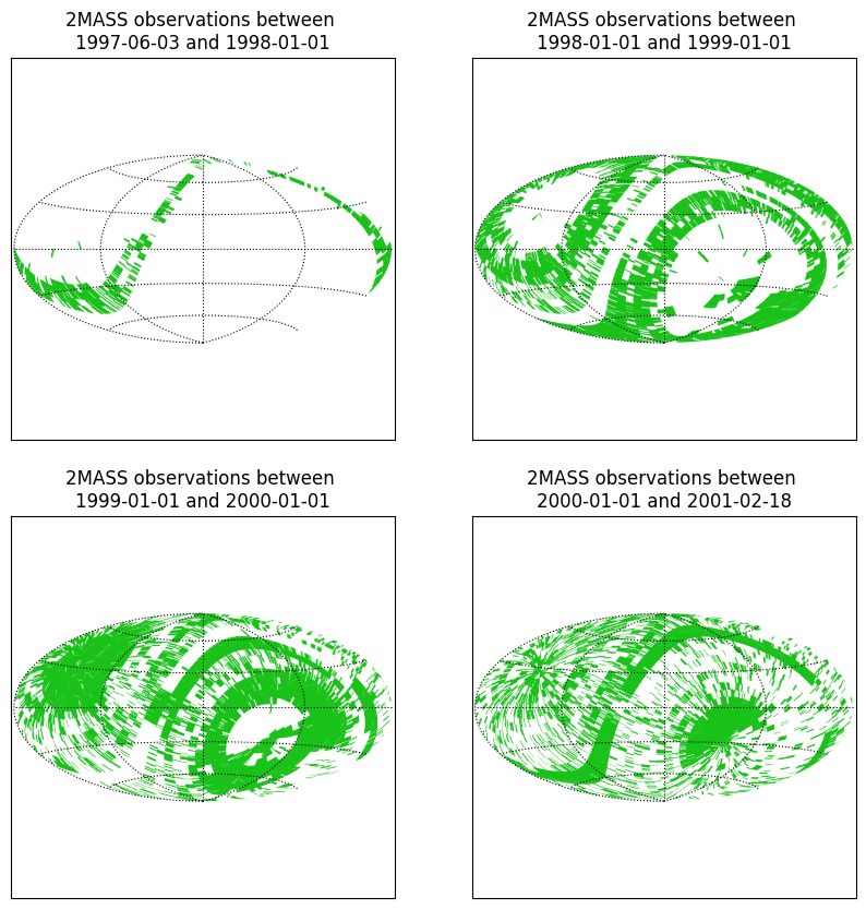
Query a ST-MOC by a time range
Let’s query the ST-MOC of 2MASS to retrieve the regions being observed each year.
[6]:
def add_to_plot(fig, label, wcs, title, moc):
    """Add a MOC to a plot."""
    ax = fig.add_subplot(label, projection=wcs)

    ax.grid(color="black", linestyle="dotted")
    ax.set_title(title)
    ax.set_xlabel("lon")
    ax.set_ylabel("lat")

    moc.fill(ax=ax, wcs=wcs, alpha=0.9, fill=True, linewidth=0, color="#00bb00")
    # moc.border(ax=ax, wcs=wcs, linewidth=1, color="green")


fig = plt.figure(figsize=(10, 10))

time_ranges = Time(
    [
        [["1997-06-03", "1998-01-01"]],
        [["1998-01-01", "1999-01-01"]],
        [["1999-01-01", "2000-01-01"]],
        [["2000-01-01", "2001-02-18"]],
    ],
    format="iso",
    scale="tdb",
    out_subfmt="date",
)
with WCS(
    fig,
    fov=330 * u.deg,
    center=SkyCoord(0, 0, unit="deg", frame="galactic"),
    coordsys="galactic",
    rotation=Angle(0, u.degree),
    projection="AIT",
) as wcs:
    for i in range(4):
        tmoc = TimeMOC.from_time_ranges(
            min_times=time_ranges[i][0, 0],
            max_times=time_ranges[i][0, 1],
            delta_t=TimeDelta(1e-6, scale="tdb", format="sec"),
        )

        moc_2mass = two_mass.query_by_time(tmoc)
        title = f"2MASS observations between \n{time_ranges[i][0, 0].iso} and {time_ranges[i][0, 1].iso}"
        id_subplot = int("22" + str(i + 1))
        add_to_plot(fig, id_subplot, wcs, title, moc_2mass)

plt.show()
Creation of the Space-Time coverage of XMM_DR8 at the depth (time, space) = 10, 7
[7]:
# Loading & preparing the data
xmm_dr8_data = Table.read("../resources/STMOC/vizier_votable.b64")
times_xmm = Time(xmm_dr8_data["MJD0"].data, format="mjd", scale="tdb")
lon_xmm = xmm_dr8_data["RA_ICRS"].quantity
lat_xmm = xmm_dr8_data["DE_ICRS"].quantity
print("Number of rows in XMM_DR8: ", lon_xmm.shape[0])
Number of rows in XMM_DR8: 531454
[8]:
%%time
# Create the STMOC
xmm_dr8_stmoc = STMOC.from_times_positions(
    times_xmm,
    time_depth,
    lon_xmm,
    lat_xmm,
    spatial_depth,
)
CPU times: user 622 ms, sys: 680 ms, total: 1.3 s
Wall time: 323 ms
2. Intersection between the 2MASS and XMM_DR8 Space-Time coverages
ST-MOCs are very convinient when it comes to perform logical operations between them (as it is already possible with spatial footprints).
As an example, it is possible to retrieve the areas that have been observed at the same time by the 2MASS and XMM survey! It benefits from the good performance of MOC (thanks to its core functions written in Rust).
[9]:
%%time
# Compute their intersection and check that it is not empty
xmm_inter_2mass = xmm_dr8_stmoc.intersection(two_mass)

print("Is the MOC intersection empty?:", xmm_inter_2mass.is_empty())

print("Time of the first observation:", xmm_inter_2mass.min_time.iso)
print("Time of the last observation:", xmm_inter_2mass.max_time.iso)
Is the MOC intersection empty?: False
Time of the first observation: 2000-02-18 06:49:16.163
Time of the last observation: 2000-11-05 03:55:44.532
CPU times: user 5.56 ms, sys: 1.51 ms, total: 7.06 ms
Wall time: 7.67 ms
3. Filter catalogs by a Space-Time coverage
ST-MOCs can be used to retrieve the sources in 2MASS and XMM_DR8 that have been observed at the same time i.e. within a ~3 days time resolution and a 27 arcsec spatial resolution.
Let’s retrieve the XMM sources being observed at the same time by 2MASS.
[10]:
%%time
# Filtering a 4.8M rows table is quite fast
mask_xmm = xmm_inter_2mass.contains(times_xmm, lon_xmm, lat_xmm)
sources_xmm = xmm_dr8_data[mask_xmm]

print(f"\n {len(sources_xmm)} sources in XMM\n")
sources_xmm
 100 sources in XMM

CPU times: user 53.8 ms, sys: 37.5 ms, total: 91.3 ms
Wall time: 98.1 ms
[10]:
| RA_ICRS | DE_ICRS | MJD0 | recno |
|---|---|---|---|
| deg | deg | d | |
| float64 | float64 | float64 | int32 |
| 54.181699 | 0.604013 | 51592.5937 | 89571 |
| 54.189898 | 0.605876 | 51592.5937 | 89593 |
| 54.197439 | 0.589064 | 51592.5937 | 89616 |
| ... | ... | ... | ... |
| 123.063435 | 75.918958 | 51852.8680 | 179052 |
| 123.172708 | 76.102680 | 51852.8680 | 179117 |
| 123.490485 | 75.910425 | 51852.8680 | 179337 |
One can then use astroquery.vizier to get more informations about the filtered sources.
[11]:
xmm_skycoords = SkyCoord(
    sources_xmm["RA_ICRS"].data,
    sources_xmm["DE_ICRS"].data,
    unit="deg",
    frame=ICRS(),
)

# Query the IX/55/xmm3r8s catalog with the three first positions + 0.1 arcsec
result = Vizier.query_region(
    xmm_skycoords[:3],
    radius=Angle(0.1, "arcsec"),
    catalog="IX/55/xmm3r8s",
)[0]
result
[11]:
| _q | 3XMM | RA_ICRS | DE_ICRS | srcML | Flux8 | e_Flux8 | HR1 | HR2 | HR3 | HR4 | ext | V | S | Nd | xcatDBdet | xcatDB | IRAP |
|---|---|---|---|---|---|---|---|---|---|---|---|---|---|---|---|---|---|
| deg | deg | mW / m2 | mW / m2 | arcsec | |||||||||||||
| int32 | str16 | float64 | float64 | float64 | float64 | float64 | float64 | float64 | float64 | float64 | float64 | uint8 | uint8 | int16 | str9 | str6 | str4 |
| 1 | J033643.6+003614 | 54.181699 | 0.604013 | 67.363 | 2.6823e-14 | 4.2254e-15 | 0.192770 | -0.010170 | -0.799786 | -1.000000 | 0.000000 | 1 | 0 | 1 | xcatDBdet | xcatDB | IRAP |
| 2 | J033645.5+003621 | 54.189898 | 0.605876 | 52.302 | 9.7142e-15 | 3.2946e-15 | 0.275784 | -0.153472 | -0.562840 | -1.000000 | 0.000000 | 1 | 1 | 1 | xcatDBdet | xcatDB | IRAP |
| 3 | J033647.3+003520 | 54.197439 | 0.589064 | 42180 | 9.7749e-12 | 1.8025e-13 | 0.372987 | 0.023216 | -0.508756 | -0.779417 | 16.185900 | 1 | 1 | 1 | xcatDBdet | xcatDB | IRAP |
4. Save into a FITS file
[12]:
xmm_inter_2mass.save("xmm_inter_2mass_stmoc.fits", format="fits", overwrite=True)
5. Vizualize a Space-Time coverage interactively
An interactive slider allows to select a time range. Whenever the slider moves, the ST-MOC is queried by the new time range. Each time query gives back the spatial footprint during that time (i.e. a mocpy.MOC object).
You can change the field of view to zoom in (resp. zoom out) if you want. By reducing the FoV you will be able to vizualize the sources in XMM filtered by the intersection Space-Time coverage.
[13]:
output = widgets.Output()


def update(change):
    """Define an interactive plot for time MOCs."""
    global t, output, time_slider
    global last_t1, last_t2
    global moc
    output.clear_output(wait=True)

    new_values = time_slider.value if change is None else change.new

    new_t1, new_t2 = new_values

    tmoc_constraint = TimeMOC.from_time_ranges(
        min_times=Time([new_t1], format="mjd", scale="tdb"),
        max_times=Time([new_t2], format="mjd", scale="tdb"),
        delta_t=TimeDelta(1e-6, scale="tdb", format="sec"),
    )
    # Query the Space-Time coverages with the same time frame
    # This operation returns a spatial coverage and is pretty fast thanks to
    # the data-structure used for storing Space-Time coverages.
    moc_2mass = two_mass.query_by_time(tmoc_constraint)
    moc_xmm_dr8 = xmm_dr8_stmoc.query_by_time(tmoc_constraint)
    moc_xmm_dr8_inter_2mass = xmm_inter_2mass.query_by_time(tmoc_constraint)

    # Plot the spatial coverages
    with output:
        fig = plt.figure(111, figsize=(15, 10))

        with WCS(
            fig,
            fov=50 * u.deg,
            center=SkyCoord(140, 30, unit="deg", frame="galactic"),
            coordsys="galactic",
            rotation=Angle(0, u.degree),
            projection="AIT",
        ) as wcs:
            ax = fig.add_subplot(1, 1, 1, projection=wcs)
            # Call fill with a matplotlib axe and the `~astropy.wcs.WCS` wcs object.
            moc_2mass.fill(
                ax=ax,
                wcs=wcs,
                alpha=0.5,
                fill=True,
                color="green",
                label="2mass",
            )
            moc_xmm_dr8.fill(
                ax=ax,
                wcs=wcs,
                alpha=0.5,
                fill=True,
                color="red",
                label="xmm_dr8",
            )
            moc_xmm_dr8_inter_2mass.fill(
                ax=ax,
                wcs=wcs,
                alpha=0.5,
                fill=True,
                color="blue",
                label="xmm_dr8 inter 2mass",
            )

            # Plot the sources contained into `xmm_inter_2mass`
            skycoords = SkyCoord(
                sources_xmm["RA_ICRS"].data,
                sources_xmm["DE_ICRS"].data,
                unit="deg",
                frame=ICRS(),
            )
            X, Y = SkyCoord.to_pixel(skycoords, wcs)
            ax.scatter(
                X,
                Y,
                color="yellow",
                alpha=1,
                marker="x",
                label="sources from XMM filtered through \nxmm_dr8 inter 2mass",
                zorder=2,
            )

            ax.legend(loc="lower left")

        plt.xlabel("GLON")
        plt.ylabel("GLAT")

        plt.title(
            "Coverage of 2MASS images, XMM_DR8 and their intersection between "
            f"MJD {new_values[0]} and {new_values[1]}",
        )
        plt.grid(color="black", linestyle="dotted")
        plt.show()
[14]:
min_time = int(np.min(two_mass_data["mjd"])) - 1
max_time = int(np.max(two_mass_data["mjd"])) + 1

time_slider = widgets.IntRangeSlider(
    value=[51594, 51917],
    min=min_time,
    max=max_time,
    step=1,
    description="MJD interval:",
    disabled=False,
    continuous_update=False,
    orientation="horizontal",
    layout={"width": "90%"},
)
[15]:
# In blue is a region that has been observed by 2MASS and XMM_DR8 at the same time
time_slider.observe(update, "value")
update(None)
widgets.VBox([time_slider, output])
[15]: