Advanced usage of MOCs to explore complex regions of interest

Stefania Amodea¹, Matthieu Baumann¹, Thomas Boch¹, Caroline Bot¹, Katarina A. Lutz¹.

1. Université de Strasbourg, CNRS, Observatoire Astronomique de Strasbourg, UMR 7550, F-67000, Strasbourg, France

Thomas Boch and Caroline Bot wrote the original version of this tutorial, available on the EURO-VO tutorials page. It was presented at the workshop “Detecting the unexpected, Discovery in the Era of Astronomically Big Data”. The version here is an adaptation to jupyter notebooks by the Strasbourg astronomical Data Center (CDS) team.

---

Introduction

I have a set of images. I would like to select regions in my observations that are above a given threshold in another survey (e.g. at low extinction), retrieve objects from very large catalogs (e.g. Gaia + 2MASS) in these non-trivial shapes and not-necessarily-connected regions, and combine them to visualize some quantities (e.g. color color diagram).

# Standard Library
from pathlib import Path

# Astronomy tools
import astropy.units as u
from astropy.coordinates import Angle, SkyCoord, match_coordinates_sky
from astropy.io import fits

# Access astronomical databases
import pyvo
from astroquery.vizier import Vizier

# Moc and HEALPix tools
import cdshealpix
import mocpy

# For plots
import matplotlib.pyplot as plt

# Data handling
import numpy as np

Step 1: Finding the images

We want to find all Short-Red images in the Macquarie/AAO/Strasbourg Hα Planetary Galactic catalog (MASH) using the VizieR associated data service.

The VizieR service at CDS inventories astronomical catalogs published in the literature. Some of these catalogs contain data associated with publications and the tables therein. This data can be browsed and explored through the VizieR-associated data service, linked to the traditional VizieR table service. Here we look for images associated with the MASH catalog of planetary nebulae (Parker et. al. 2006-2008). The MASH fits files are cut-outs extracted from a larger Hα and Short Red survey to constitute a set of regions of interest around planetary nebulae.

To find VizieR-associated data, we use the Table Access Protocol (TAP) with the VizieR endpoint. Through the VizieR TAP endpoint, we can search for tables, their content, and information on associated data.

First, we search for the MASH catalog:

# give the address of the service, you can also directly visit the website
tap_vizier = pyvo.dal.TAPService("https://tapvizier.cds.unistra.fr/TAPVizieR/tap")

# a query that searches for all tables with the words MASH and Parker in their description
query = """
        SELECT  *  FROM tables 
        WHERE description LIKE '%MASH%Parker%'
        """

mash_catalogues = tap_vizier.search(query).to_table()
mash_catalogues

Table length=5

schema_name	table_name	table_type	description	utype	nrows
object	object	object	object	object	object
J_MNRAS	J/MNRAS/412/223/table4	table	The nine MASH PNe detected and possibly detected in the PMN survey ( Bojicic I.S., Parker Q.A., Filipovic M.D., Frew D.J.)		9
J_MNRAS	J/MNRAS/412/223/table1	table	MASH PNe detected in the NVSS ( Bojicic I.S., Parker Q.A., Filipovic M.D., Frew D.J.)		201
V_combined	V/127A/mash2	table	The MASH-II Supplement (from paper II) ( Parker Q.A., Acker A., Frew D.J., Hartley M., Peyaud A.E.J., Phillipps S., Russeil D., Beaulieu S.F., Cohen M., Koppen J., Marcout J., Miszalski B., Morgan D.H., Morris R.A.H., Ochsenbein F., Pierce M.J.,)		335
V_combined	V/127A/mash1	table	The MASH Catalog of Planetary Nebulae (paper I) ( Parker Q.A., Acker A., Frew D.J., Hartley M., Peyaud A.E.J., Phillipps S., Russeil D., Beaulieu S.F., Cohen M., Koppen J., Marcout J., Miszalski B., Morgan D.H., Morris R.A.H., Ochsenbein F., Pierce M.J.,)		903
J_MNRAS	J/MNRAS/412/223/mpgs2	table	MASH PNe detected in the MPGS-2 (Cat. VIII/82) ( Bojicic I.S., Parker Q.A., Filipovic M.D., Frew D.J.)		81

In this tutorial, we are interested in the tables belonging to the catalogs V/127A. This includes tables V/127A/mash1 and V/127A/mash2. To have a look at the content of these tables, we look at their first lines like this:

query = """
        SELECT TOP 5 * FROM \"V/127A/mash1\" 
        """
mash1_head = tap_vizier.search(query).to_table()
mash1_head

Table length=5

recno	n_PNG	PNG	Name	RAJ2000	DEJ2000	GLon	GLat	MajDiam	MinDiam	CS	Morph	Tel	ObsDate	HaExp	HaFld	Comments	img	ImageHa	ImageSr	AssocData
				deg	deg	deg	deg	arcsec	arcsec				'Y:M:D'
int32	str1	object	object	float64	float64	float64	float64	float64	float64	object	object	object	float64	object	object	object	object	object	object	object
29	L	G234.7-02.2	PHR0724-2021	111.05458333333331	-20.36361111111111	234.7045	-2.2774	134.5	54.0		A	SA	2452672.0	HA18201	HA842	Large, very faint diffuse arcuate nebula; has [NII]~2xH-alpha, nothing in blue	1029	img_ha	img_sr	fits
2	P	G227.3-12.0	PHR0633-1808	98.35374999999999	-18.13972222222222	227.3207	-12.0289	17.0	15.0		Ea	SA	2452672.0	HA18191	HA926	Very faint, partial arcuate nebula also observed M1 060100; [NII]~0.8xH-alpha, strong [SII], only weak H-beta in blue - inconclusive	1002	img_ha	img_sr	fits
16	T	G227.2-03.4	PHR0705-1419	106.41041666666665	-14.318055555555553	227.2852	-3.4029	15.0	15.0		E	SA	2452668.0	HA18244	HA1017	Small, circular PN around a faint central star; also observed M1 040100; [NII]~0.7 H-alpha, [OIII]>>H-beta	1016	img_ha	img_sr	fits
5	L	G223.6-06.8	PHR0646-1235	101.60583333333332	-12.598888888888887	223.6338	-6.8035	40.0	37.0		E	SA	2453788.0	HA18194	HA1016	Slightly oval very faint PN candidate - has [OIII] and H-alpha	1005	img_ha	img_sr	fits
10	P	G224.3-05.5	PHR0652-1240	103.08458333333331	-12.67611111111111	224.3504	-5.5463	187.0	180.0		I	SA	2452670.0	HA18244	HA1017	Faint, extended S-shaped emission nebula, possible evolved PN, also observed M1 080100; has [NII]~0.8Ha, [OIII], strong [SII], [OIII]>H-beta	1010	img_ha	img_sr	fits

As you can see, the last column of this table is called AssocData and contains the entry fits. If you look at this table on the VizieR web interface, you can download the associated fits file. Within this notebook, we query the obscore database to get the URLs to the fits file. Using the astropy.io.fits module, we can open the fits files from their URLs.

obs_tap_vizier = pyvo.dal.TAPService(
    "https://cdsarc.cds.unistra.fr/saadavizier.tap/tap",
)
query = """
        SELECT TOP 5  *  FROM obscore 
        WHERE obs_collection='V/127A'   
        """
mash_fits = obs_tap_vizier.search(query).to_table()
mash_fits

Table length=5

access_estsize	access_format	access_url	bib_reference	calib_level	dataproduct_type	em_band	em_max	em_min	extension	facility_name	has_wcs	instrument_name	obs_collection	obs_id	obs_publisher_did	oidsaada	o_ucd	pol_states	s_dec	s_fov	s_ra	s_region	s_resolution	target_name	t_exptime	t_max	t_min	t_resolution
kbyte						spect			meta.code		meta.code								deg	deg	deg		arcsec
int64	object	object	object	int32	object	object	float64	float64	int32	object	int32	object	object	object	object	object	object	object	float64	float64	float64	object	float64	object	float64	float64	float64	float64
610	application/fits	https://cdsarc.cds.unistra.fr/saadavizier/download?oid=864975549779410945	2006MNRAS.373...79P	-1	image	Optical	1e-06	3e-07	--	UKST	5	SuperCOSMOS I	V/127A	1032_sr.fits	ivo://CDS.VizieR/V/127A?res=1032_sr.fits	864975549779410945	obs.image	NotSet	-13.784389854801203	0.0713021682865721	111.43275777455307	Polygon ICRS 111.46664940645094 -13.81781914701963 111.39832407190251 -13.817324215795937 111.3988758446347 -13.750955924906409 111.46718176614709 -13.751450706358609	0.948991575097523		--	--	51226.0	--
714	application/fits	https://cdsarc.cds.unistra.fr/saadavizier/download?oid=864975549779410946	2006MNRAS.373...79P	-1	image	Optical	1e-06	3e-07	--	UKST	5	SuperCOSMOS I	V/127A	1002_ha.fits	ivo://CDS.VizieR/V/127A?res=1002_ha.fits	864975549779410946	obs.image	NotSet	-18.139618250252592	0.06807629850604295	98.3536194209876	Polygon ICRS 98.3879823237976 -18.17328539691655 98.31817068063498 -18.172295336426327 98.31926974725019 -18.105945008699248 98.38905491554986 -18.106934677663524	0.9487309062128839		--	--	51158.0	--
754	application/fits	https://cdsarc.cds.unistra.fr/saadavizier/download?oid=864975549779410947	2006MNRAS.373...79P	-1	image	Optical	1e-06	3e-07	--	UKST	5	SuperCOSMOS I	V/127A	1033_ha.fits	ivo://CDS.VizieR/V/127A?res=1033_ha.fits	864975549779410947	obs.image	NotSet	-28.97290230510999	0.07273587908530431	111.5198237403422	Polygon ICRS 111.55713579830989 -29.006593110324985 111.48129478490598 -29.005543503560524 111.48253597444139 -28.939201209841514 111.5583283925454 -28.94025013401036	0.9486651876518051		--	--	50867.0	--
581	application/fits	https://cdsarc.cds.unistra.fr/saadavizier/download?oid=864975549779410948	2006MNRAS.373...79P	-1	image	Optical	1e-06	3e-07	--	UKST	5	SuperCOSMOS I	V/127A	1002_sr.fits	ivo://CDS.VizieR/V/127A?res=1002_sr.fits	864975549779410948	obs.image	NotSet	-18.13962593857754	0.06807301936327177	98.35359006999442	Polygon ICRS 98.38795041597254 -18.17329148584167 98.31813924430983 -18.172303630142665 98.31924295149577 -18.105954297342016 98.38902764888365 -18.106941759807857	0.9487205770226425		--	--	51160.0	--
607	application/fits	https://cdsarc.cds.unistra.fr/saadavizier/download?oid=864975549779410949	2006MNRAS.373...79P	-1	image	Optical	1e-06	3e-07	--	UKST	5	SuperCOSMOS I	V/127A	1033_sr.fits	ivo://CDS.VizieR/V/127A?res=1033_sr.fits	864975549779410949	obs.image	NotSet	-28.97292411093542	0.07273534143391176	111.51984609001715	Polygon ICRS 111.55715777828372 -29.00661467563269 111.48131691638382 -29.005565388666998 111.48255869339395 -28.93922325635545 111.55835096020016 -28.940271860424208	0.9486629846629874		--	--	50879.0	--

As you can see, the result from this query provides information on the fits files associated with the MASH catalogs. In particular, the column access_url provides the location of the data. To get the first image we can do:

# download the first image
hdul_list = fits.open(mash_fits["access_url"][0])

# plot it in a quick preview
plt.imshow(hdul_list[0].data, cmap="gray", origin="lower")

<matplotlib.image.AxesImage at 0x7f080586ebb0>

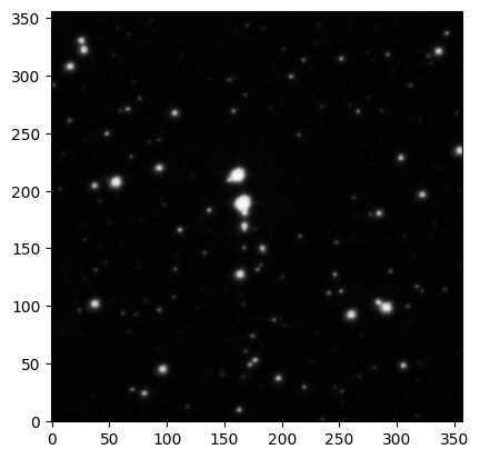
This should be done for every image in the list. However, downloading all the data takes quite some time. For this tutorial, we prepared a subsample of 335 of these Short Red images that will run promptly but we encourage you to try accessing the full Short Red sample on your own later. The subsample is available in the Data Folder of this repository.

Step 2: Create a MOC of the MASH images

The multi-order coverage (MOC) map of a set of images represents their sky coverage. MOCs can describe arbitrary zones in the sky which do not need to be connected. You’ll see that the union or intersection of two MOCs requires few time and computational effort. Catalogs can also be filtered by MOCs.

Here we want to use the fits files just downloaded to create a MOC map corresponding to the coverage of the MASH images.

Organising data

# Where to find fits images downloaded from the archive above
datadir = Path("Data/MASH_Sample/")
datadir.mkdir(parents=True, exist_ok=True)

In most cases, we could ignore the next cell. However, some possible deprecated keywords in the fits header would hamper the MOC creation and would cause errors in the underlying astropy.wcs.WCS module. This is why we rewrite the headers of the fits files so that they only contain the useful keywords needed to define the coordinate frame correctly before using mocpy.

Create the MOC

Here we can create the MOC of the MASH images with the MOCPy module. This can take a few seconds.

# Get a list of the fits files and create the MOC
mash_file_list = datadir.glob(
    "*_sr_modified.fits",
)  # glob allows to find all paths that end with _sr_modified.fits in datadir
mash_file_list = [str(file_path) for file_path in mash_file_list]
moc_mash = mocpy.MOC.from_fits_images(mash_file_list, max_norder=15)
# this takes a bit of time because a lot of files are opened and processed to extract the moc

WARNING: FITSFixedWarning: RADECSYS= 'FK5 ' 
the RADECSYS keyword is deprecated, use RADESYSa. [astropy.wcs.wcs]

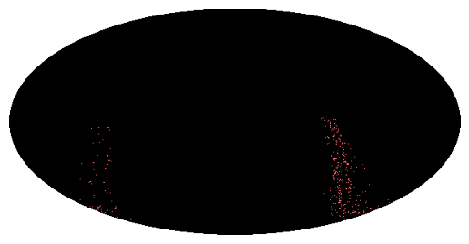
Plot the MOC

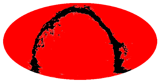
We can chose between two of the MOCpy methods to plot the MOC

# A one-liner for a very fast visualization
moc_mash.display_preview()

# With a bit more control over the output, the MOC.wcs method
fig = plt.figure(figsize=(10, 7))
wcs = moc_mash.wcs(fig)
ax = fig.add_subplot(projection=wcs)
ax.grid(True)  # noqa: FBT003
moc_mash.fill(ax, wcs, color="purple", alpha=0.5)

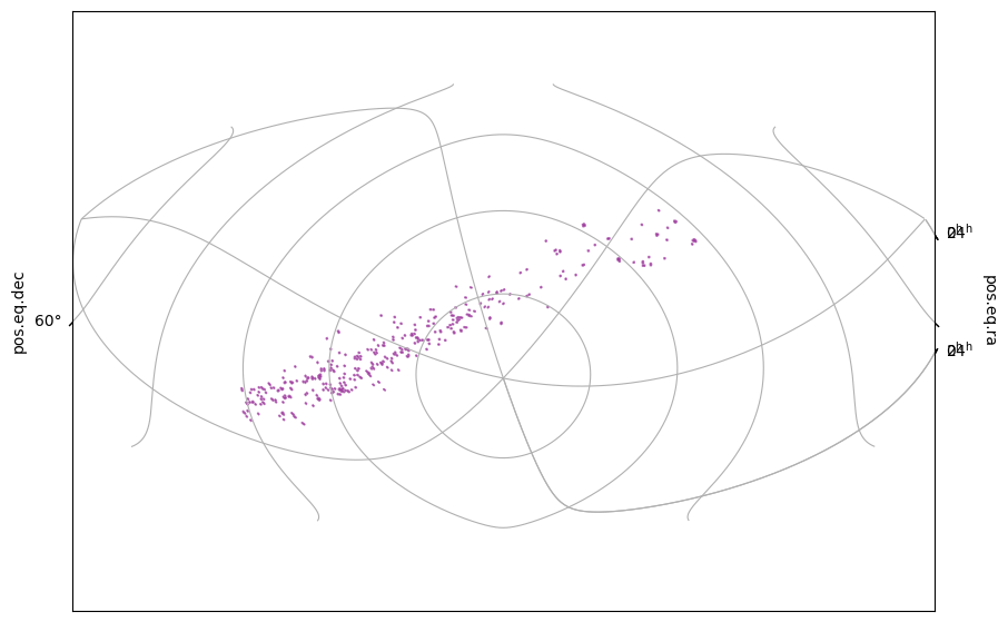
You can see how the MOC has arbitrary shapes and not all regions are connected.

And for more control over the plot parameters, there is also the mocpy.WCS method (!)

Step 3: Load an archival extinction map and create the MOC of the low extinction regions

Different works (e.g. Schlegel et al. 1998, Schlafly & Finkbeiner 2011, Green et al. 2015…) have created extinction maps of the sky that are publicly available. Some of these maps are all-sky maps, while others have higher resolutions, or come from different methods… They can be found in HEALPix format (among others) on the Legacy Archive for Microwave Background Data Analysis (LAMBDA) website or on the Analysis Center for Extended Data (CADE) website.

For this tutorial, we will download the well-known all-sky extinction map from Schlegel et al. from the LAMBDA website and define the low extinction area for which \(0 < E(B-V) < 0.5\) as a MOC. It has an information page.

The map is available here: https://lambda.gsfc.nasa.gov/data/foregrounds/SFD/lambda_sfd_ebv.fits and we save it to disc.

hdul = fits.open(
    "https://lambda.gsfc.nasa.gov/data/foregrounds/SFD/lambda_sfd_ebv.fits",
)

We are only interested in regions with low extinction. So we aim to get a MOC of all regions where the extinction values from the Schlegel et al. map are between 0 and 0.5mag. The extinction map we got from the NASA webpage is in the HEALPix format. This is an efficient presentation of all-sky maps. The HEALPix tesselation is also used by MOCs. So to get the MOC from the extinction map, we do the following.

First, we check the coordinate system in the map header. We will need to convert to equatorial coordinates, change the projection of the map, and set the order (i.e. resolution) of the map.

hdr = hdul[0].header
hdr

SIMPLE  =                    T / file does conform to FITS standard             
BITPIX  =                   32 / number of bits per data pixel                  
NAXIS   =                    0 / number of data axes                            
EXTEND  =                    T / FITS dataset may contain extensions            
COMMENT   FITS (Flexible Image Transport System) format is defined in 'Astronomy
COMMENT   and Astrophysics', volume 376, page 359; bibcode: 2001A&A...376..359H 
DATE    = '2003-02-05T00:00:00' /file creation date (YYYY-MM-DDThh:mm:ss UT)    
OBJECT  = 'ALL-SKY '           / Portion of sky given                           
COMMENT   This file contains an all-sky Galactic reddening map, E(B-V), based on
COMMENT   the derived reddening maps of Schlegel, Finkbeiner and Davis (1998).  
COMMENT   Software and data files downloaded from their website were used to    
COMMENT   interpolate their high resolution dust maps onto pixel centers        
COMMENT   appropriate for a HEALPix Nside=512 projection in Galactic            
COMMENT   coordinates. This file is distributed and maintained by LAMBDA.       
REFERENC= 'Legacy Archive for Microwave Background Data Analysis (LAMBDA)      '
REFERENC= '                http://lambda.gsfc.nasa.gov/                        '
REFERENC= 'Maps of Dust Infrared Emission for Use in Estimation of Reddening an'
REFERENC= ' Cosmic Microwave Background Radiation Foregrounds',                '
REFERENC= ' Schlegel, Finkbeiner & Davis 1998 ApJ 500, 525                     '
REFERENC= 'Berkeley mirror site for SFD98 data: http://astron.berkeley.edu/dust'
REFERENC= 'Princeton mirror site for SFD98 data:                               '
REFERENC= '                           http://astro/princeton.edu/~schlegel/dust'
REFERENC= 'HEALPix Home Page: http://www.eso.org/science/healpix/              '
RESOLUTN=                    9 / Resolution index                               
SKYCOORD= 'Galactic'           / Coordinate system                              
PIXTYPE = 'HEALPIX '           / Pixel algorithm                                
ORDERING= 'NESTED  '           / Ordering scheme                                
NSIDE   =                  512 / Resolution parameter                           
NPIX    =              3145728 / # of pixels                                    
FIRSTPIX=                    0 / First pixel (0 based)                          
LASTPIX =              3145727 / Last pixel (0 based)                           

print((hdul[1].data).shape)
hdul[1].data

(3145728,)

FITS_rec([( 9.625492, 1.), (46.090515, 1.), ( 8.18071 , 1.), ...,
          (15.149189, 1.), (14.107367, 1.), (15.463686, 1.)],
         dtype=(numpy.record, [('TEMPERATURE', '>f4'), ('N_OBS', '>f4')]))

The data field here has a specific shape. It contains tuples for which the first value is the extinction (named ‘TEMPERATURE’) and the second one is the number of observations of the value (you can check that it is 1 everywhere).

extinction_values = hdul[1].data["TEMPERATURE"]

Let’s extract the information about the number of sides and the order of the healpix map from the header of the fits file

nside = hdul[0].header["NSIDE"]
norder = hdul[0].header["RESOLUTN"]

The header allows to see that this map is in galactic coordinates. We will need to convert this into equatorial coordinates to compare with our other maps.

# Creation of an HEALpix grid at order 9 in nested ordering
healpix_index = np.arange(12 * 4**norder, dtype=np.uint64)
print(
    f"We can check the the NPIX value corresponds to the one in the header here: {len(healpix_index)}",
)

We can check the the NPIX value corresponds to the one in the header here: 3145728

# Get the coordinates of the centers of these healpix cells
center_coordinates_in_equatorial = cdshealpix.healpix_to_skycoord(
    healpix_index,
    depth=9,
)
center_coordinates_in_equatorial

<SkyCoord (ICRS): (ra, dec) in deg
    [( 45.        ,  0.0746039 ), ( 45.08789062,  0.14920793),
     ( 44.91210938,  0.14920793), ..., (315.08789062, -0.14920793),
     (314.91210938, -0.14920793), (315.        , -0.0746039 )]>

# Convert this into galactic coordinates
center_coordinates_in_galactic = center_coordinates_in_equatorial.galactic
center_coordinates_in_galactic

<SkyCoord (Galactic): (l, b) in deg
    [(176.8796283 , -48.85086427), (176.89078038, -48.7358142 ),
     (176.70525363, -48.86216423), ..., ( 48.82487228, -28.4122831 ),
     ( 48.7216889 , -28.26178141), ( 48.84578935, -28.29847774)]>

# Calculate the bilinear interpolation we must apply to each healpix cell to get the values in the other coordinate system
healpix, weights = cdshealpix.bilinear_interpolation(
    center_coordinates_in_galactic.l,
    center_coordinates_in_galactic.b,
    depth=norder,
)

# Apply the interpolation
ext_map_equatorial_nested = (extinction_values[healpix.data] * weights.data).sum(axis=1)
ext_map_equatorial_nested

array([0.08981742, 0.0991632 , 0.08249644, ..., 0.08323811, 0.08352184,
       0.0820533 ])

Next we declare which pixel we want to use, let’s take all pixels with an extinction lower than 0.5:

low_extinction_index = np.where(ext_map_equatorial_nested < 0.5)[0]
print(
    f"The low extinction criteria keeps {round((len(low_extinction_index)/ len(extinction_values)*100), 2)}% of the sky map",
)

The low extinction criteria keeps 86.74% of the sky map

And let’s create a MOC from this criteria

moc_low_extinction = mocpy.MOC.from_healpix_cells(
    low_extinction_index,
    np.full(
        (
            len(
                low_extinction_index,
            )
        ),
        norder,
    ),
    norder,
)

Step 4: Find out which regions are covered by the MASH short-red images in the low extinction regions defined above

To find out the sky regions of the MASH sample that are at low extinction, we build the intersection of the two MOCs.

moc_intersection = moc_low_extinction.intersection(moc_mash)
# Once the intersection is bluit, we can for example print the sky fraction :
print(
    f"The intersection of the two MOCs covers {round(moc_intersection.sky_fraction * 100, 4)}% of the sky",
)

The intersection of the two MOCs covers 0.4778% of the sky

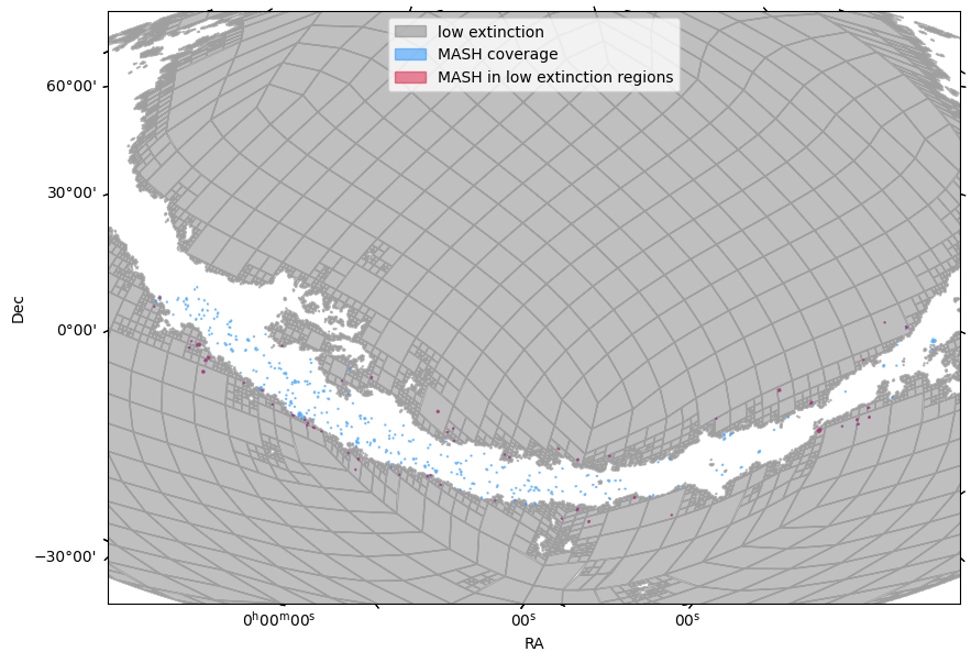
Now we can visualize the coverage of the two MOCs and their intersection. The grey area is where the extinction is low. The blue one is the MASH coverage. The tiny red dots show the MASH coverage in low extinction regions.

fig = plt.figure(111, figsize=(10, 7))

with mocpy.WCS(
    fig,
    fov=140 * u.deg,
    center=SkyCoord(200, -20, unit="deg", frame="icrs"),
    coordsys="icrs",
    rotation=Angle(0, u.degree),
    projection="AIT",
) as wcs:
    ax = fig.add_subplot(1, 1, 1, projection=wcs)

    moc_low_extinction.fill(
        ax=ax,
        wcs=wcs,
        alpha=0.5,
        fill=True,
        color="grey",
        label="low extinction",
    )
    moc_mash.fill(
        ax=ax,
        wcs=wcs,
        alpha=0.5,
        fill=True,
        color="dodgerblue",
        label="MASH coverage",
    )
    moc_intersection.fill(
        ax=ax,
        wcs=wcs,
        alpha=0.5,
        fill=True,
        color="crimson",
        label="MASH in low extinction regions",
    )
    # Sets labels
    ax.set_xlabel("RA")
    ax.set_ylabel("Dec")
    # Sets ticks
    lon, lat = ax.coords[0], ax.coords[1]
    lon.set_major_formatter("hh:mm:ss")
    lat.set_major_formatter("dd:mm")
    lon.set_ticklabel(exclude_overlapping=True)
    lat.set_ticklabel(exclude_overlapping=True)
plt.legend()

<matplotlib.legend.Legend at 0x7f08011ea3a0>

Step 5: Query the 2MASS and Gaia Catalogues by MOC

Without the usage of MOC, querying for sources in the low extinction regions covered by the MASH subsample would be tedious or even impossible. Indeed, one would need to load the whole catalog and make selections which would not be possible given the size of some catalogs. Alternatively, one would need to query the catalog field by field, which would take time and several queries. Instead, here we will use the power of MOC files to query large catalogs directly in the covered regions only. We will use coverages of the low extinction and MASH regions to query for sources from the Gaia and 2MASS surveys in these highly non-continuous and non-trivial shape areas.

First, let’s see which Gaia and 2MASS catalogs are available on VizieR. We could, as above, use the TAP endpoint of VizieR. But we show below the Vizier module in the astroquery package.

catalog_list_twomass = Vizier.find_catalogs("Cutri")
for k, v in catalog_list_twomass.items():
    print(k, ": ", v.description)

II/126 :  IRAS Serendipitous Survey Catalog (IPAC 1986)
II/241 :  2MASS Catalog Incremental Data Release (IPAC/UMass, 2000)
II/246 :  2MASS All-Sky Catalog of Point Sources (Cutri+ 2003)
II/281 :  2MASS 6X Point Source Working Database / Catalog (Cutri+ 2006)
II/307 :  WISE Preliminary Data Release (Cutri+ 2011)
II/311 :  WISE All-Sky Data Release (Cutri+ 2012)
II/328 :  AllWISE Data Release (Cutri+ 2013)
II/365 :  The CatWISE2020 catalog (updated version 28-Jan-2021) (Marocco+, 2021)
VII/233 :  2MASS All-Sky Extended Source Catalog (XSC) (IPAC/UMass, 2003-2006)
J/ApJ/560/566 :  K-band galaxy luminosity function from 2MASS (Kochanek+, 2001)
J/ApJ/564/421 :  Spectra of T dwarfs. I. (Burgasser+, 2002)
J/ApJ/569/23 :  Optical polarisation of 2MASS QSOs (Smith+, 2002)
J/ApJ/635/214 :  Chandra X-ray sources and NIR identifications (Ebisawa+, 2005)
J/ApJ/713/330 :  Spitzer observations of major-merger galaxies (Xu+, 2010)
J/ApJ/719/550 :  Deep NIR imaging of {rho} Oph cloud core (Marsh+, 2010)
J/ApJ/741/68 :  Main Belt asteroids with WISE/NEOWISE. I. (Masiero+, 2011)
J/ApJ/742/40 :  Jovian Trojans asteroids with WISE/NEOWISE (Grav+, 2011)
J/ApJ/743/156 :  NEOWISE observations of NEOs: preliminary results (Mainzer+, 2011)
J/ApJ/744/197 :  WISE/NEOWISE observations of Hilda asteroids (Grav+, 2012)
J/ApJ/759/L8 :  WISE/NEOWISE observations of main belt asteroids (Masiero+, 2012)
J/ApJ/760/L12 :  WISE/NEOWISE NEOs preliminary thermal fits (Mainzer+, 2012)
J/ApJ/780/92 :  Light curves of the RR Lyr SDSS J015450.17+001500.7 (Szabo+, 2014)
J/ApJ/783/122 :  AllWISE motion survey (Kirkpatrick+, 2014)
J/ApJ/784/110 :  NEOWISE observations of 105 near-Earth objects (Mainzer+, 2014)
J/ApJ/792/30 :  NEOWISE magnitudes for near-Earth objects (Mainzer+, 2014)
J/ApJ/805/90 :  WISE ELIRGs and comparison with QSOs (Tsai+, 2015)
J/ApJ/814/117 :  NEOWISE Reactivation mission: 1st yr data (Nugent+, 2015)
J/ApJ/874/82 :  Follow-up photometry & spectroscopy of PTF14jg (Hillenbrand+, 2019)
J/ApJS/95/1 :  Atlas of Quasar Energy Distributions (Elvis+ 1994)
J/ApJS/172/663 :  Infrared observations of the Pleiades (Stauffer+, 2007)
J/ApJS/175/191 :  Variables from 2MASS calibration fields (Plavchan+, 2008)
J/ApJS/190/100 :  NIR proper motion survey using 2MASS (Kirkpatrick+, 2010)
J/ApJS/199/26 :  The 2MASS Redshift Survey (2MRS) (Huchra+, 2012)
J/ApJS/224/36 :  The AllWISE motion survey (AllWISE2) (Kirkpatrick+, 2016)
J/ApJS/234/23 :  The WISE AGN candidates catalogs (Assef+, 2018)
J/AJ/112/62 :  Quasar absorption-line systems (Tanner+ 1996)
J/AJ/125/2521 :  2MASS6x survey of the Lockman Hole (Beichman+, 2003)
J/AJ/126/63 :  Host galaxies of 2MASS-QSOs with z<=3 (Hutchings+, 2003)
J/AJ/127/646 :  Unbiased census of AGN in 2MASS (Francis+, 2004)
J/AJ/135/2245 :  Absolute spectrum of the Sun and Vega for 0.2-30um (Rieke+, 2008)
J/AJ/144/148 :  Infrared photometry of brown dwarf and Hyper-LIRG (Griffith+, 2012)
J/AJ/152/63 :  NEOWISE reactivation mission: 2nd yr data (Nugent+, 2016)
J/AJ/154/53 :  WISE/NEOWISE observations of comets (Bauer+, 2017)
J/AJ/154/168 :  NEOWISE: thermal model fits for NEOs and MBAs (Masiero+, 2017)
J/AJ/156/60 :  Thermal model fits for short-arc NEOs with NEOWISE (Masiero+, 2018)
J/PASP/113/10 :  Sub-mJy radio sources complete sample (Masci+, 2001)

catalog_list_gaia = Vizier.find_catalogs("Gaia DR2", max_catalogs=1000)
for k, v in catalog_list_gaia.items():
    print(k, ": ", v.description)

I/324 :  The Initial Gaia Source List (IGSL) (Smart, 2013)
I/337 :  Gaia DR1 (Gaia Collaboration, 2016)
I/345 :  Gaia DR2 (Gaia Collaboration, 2018)
I/347 :  Distances to 1.33 billion stars in Gaia DR2 (Bailer-Jones+, 2018)
I/350 :  Gaia EDR3 (Gaia Collaboration, 2020)
I/352 :  Distances to 1.47 billion stars in Gaia EDR3 (Bailer-Jones+, 2021)
I/355 :  Gaia DR3 Part 1. Main source (Gaia Collaboration, 2022)
I/356 :  Gaia DR3 Part 2. Extra-galactic (Gaia Collaboration, 2022)
I/357 :  Gaia DR3 Part 3. Non-single stars (Gaia Collaboration, 2022)
I/358 :  Gaia DR3 Part 4. Variability (Gaia Collaboration, 2022)
I/359 :  Gaia DR3 Part 5. Solar System (Gaia Collaboration, 2022)
I/360 :  Gaia DR3 Part 6. Performance verification (Gaia Collaboration, 2022)
I/361 :  Gaia Focused Product Release (Gaia FPR) (Gaia Collaboration, 2023)
IV/36 :  Gaia-IPHAS/KIS Value-Added Catalogues (Scaringi+, 2018)
V/149 :  LAMOST DR2 catalogs (Luo+, 2016)
VI/137 :  GaiaSimu Universe Model Snapshot (Robin+, 2012)
VI/145 :  ASC Gaia Attitude Star Catalog (Smart, 2015)
IX/52 :  XXL Survey. DR2 (Chiappetti+, 2018)
J/A+A/523/A48 :  Gaia photometry (Jordi+, 2010)
J/A+A/634/A133 :  X-Shooter Spectral Library (XSL). DR2 (Gonneau+, 2020)
J/A+A/674/A25 :  Gaia DR3. spurious signals (Holl+, 2023)

For 2MASS we will want to use II/246 :  2MASS All-Sky Catalog of Point Sources (Cutri+ 2003) and for Gaia I/345 :  Gaia DR2 (Gaia Collaboration, 2018). Before we query the full two tables we only look at a few sources for each table to understand which columns are available. The query below will give us 50 sources each – the default for the get_catalogs method.

test_twomass = Vizier.get_catalogs("II/246")
print(test_twomass)
test_twomass[0]

TableList with 1 tables:
	'0:II/246/out' with 15 column(s) and 50 row(s) 

Table length=50

RAJ2000	DEJ2000	2MASS	Jmag	e_Jmag	Hmag	e_Hmag	Kmag	e_Kmag	Qflg	Rflg	Bflg	Cflg	Xflg	Aflg
deg	deg		mag	mag	mag	mag	mag	mag
float64	float64	str17	float32	float32	float32	float32	float32	float32	str3	int16	int16	str3	uint8	uint8
29.885839	56.739094	01593260+5644207	16.074	0.111	15.612	0.141	15.603	0.185	BBC	999	999	ccc	0	0
29.889511	56.741344	01593348+5644288	15.504	0.059	14.870	0.072	14.846	0.084	AAA	999	999	000	0	0
29.895820	56.744549	01593499+5644403	17.312	0.206	16.163	0.202	15.963	0.235	DCD	999	999	000	0	0
29.888912	56.748875	01593333+5644559	16.748	0.142	16.217	0.205	16.200	--	BDU	999	999	000	0	0
29.905339	56.747322	01593728+5644503	14.288	0.030	13.960	0.045	13.980	0.042	AAA	999	999	000	0	0
29.903272	56.754421	01593678+5645159	14.886	0.044	14.609	0.058	14.582	0.076	AAA	999	999	000	0	0
29.899930	56.755199	01593598+5645187	16.514	0.136	15.726	--	15.545	--	BUU	999	999	c00	0	0
29.915697	56.755924	01593976+5645213	16.371	0.098	15.491	0.108	15.484	0.154	ABC	999	999	000	0	0
29.902598	56.757378	01593662+5645265	16.066	0.096	15.573	0.131	15.048	0.106	ABB	999	999	000	0	0
29.891583	56.759617	01593397+5645346	15.707	0.054	15.658	0.116	15.225	0.126	ABB	999	999	000	0	0
29.897577	56.761745	01593541+5645422	16.729	0.129	16.915	--	16.512	--	BUU	999	999	000	0	0
29.895653	56.764652	01593495+5645527	15.645	0.056	15.219	0.093	15.234	0.126	AAB	999	999	000	0	0
29.875278	56.751507	01593006+5645054	16.741	0.138	16.123	0.203	16.141	--	BCU	999	999	000	0	0
...	...	...	...	...	...	...	...	...	...	...	...	...	...	...
29.932745	56.766003	01594385+5645576	14.479	0.030	13.907	0.041	13.676	0.040	AAA	999	999	000	0	0
29.928545	56.768829	01594285+5646077	14.804	0.039	14.446	0.050	14.365	0.069	AAA	999	999	000	0	0
29.932344	56.771584	01594376+5646177	15.529	0.065	15.177	0.083	15.128	0.125	AAB	999	999	000	0	0
29.931232	56.770348	01594349+5646132	16.874	0.147	16.280	0.223	15.814	0.203	BDD	999	999	cc0	0	0
29.941658	56.772991	01594599+5646227	13.444	0.027	12.788	0.034	12.698	0.022	AAA	999	999	000	0	0
29.975617	56.764015	01595414+5645504	15.050	0.046	14.759	0.055	14.512	0.068	AAA	999	999	0c0	0	0
29.977029	56.765244	01595448+5645548	16.570	0.128	16.113	0.196	15.698	--	BCU	999	999	cc0	0	0
29.976605	56.767006	01595438+5646012	16.721	0.151	16.118	0.214	15.654	0.199	BCC	999	999	0c0	0	0
29.965056	56.771534	01595161+5646175	15.803	0.060	15.462	0.098	14.942	0.104	AAA	999	999	000	0	0
29.977475	56.775036	01595459+5646301	16.744	0.136	16.131	--	15.563	--	BUU	999	999	000	0	0
29.982245	56.774803	01595573+5646292	16.129	0.092	15.912	0.159	15.960	0.244	ACD	999	999	000	0	0
29.984032	56.776730	01595616+5646362	16.772	0.120	16.815	--	15.967	0.249	BUD	999	999	000	0	0
29.970564	56.781158	01595293+5646521	15.914	0.081	15.384	0.095	15.643	0.188	AAC	999	999	000	0	0

test_gaia = Vizier.get_catalogs("I/345")
print(test_gaia)
test_gaia[0]

TableList with 20 tables:
	'0:I/345/gaia2' with 32 column(s) and 50 row(s) 
	'1:I/345/rvstdcat' with 30 column(s) and 50 row(s) 
	'2:I/345/rvstdmes' with 7 column(s) and 50 row(s) 
	'3:I/345/allwise' with 2 column(s) and 50 row(s) 
	'4:I/345/iers' with 2 column(s) and 50 row(s) 
	'5:I/345/cepheid' with 23 column(s) and 50 row(s) 
	'6:I/345/rrlyrae' with 21 column(s) and 50 row(s) 
	'7:I/345/lpv' with 11 column(s) and 50 row(s) 
	'8:I/345/varres' with 7 column(s) and 50 row(s) 
	'9:I/345/shortts' with 9 column(s) and 50 row(s) 
	'10:I/345/tsstat' with 13 column(s) and 50 row(s) 
	'11:I/345/numtrans' with 4 column(s) and 50 row(s) 
	'12:I/345/transits' with 20 column(s) and 50 row(s) 
	'13:I/345/rm' with 9 column(s) and 50 row(s) 
	'14:I/345/rmseg' with 16 column(s) and 50 row(s) 
	'15:I/345/rmout' with 2 column(s) and 50 row(s) 
	'16:I/345/ssoobj' with 6 column(s) and 50 row(s) 
	'17:I/345/ssoorb' with 19 column(s) and 50 row(s) 
	'18:I/345/ssores' with 10 column(s) and 50 row(s) 
	'19:I/345/ssoobs' with 7 column(s) and 50 row(s) 

Table length=50

RA_ICRS	e_RA_ICRS	DE_ICRS	e_DE_ICRS	Source	Plx	e_Plx	pmRA	e_pmRA	pmDE	e_pmDE	Dup	FG	e_FG	Gmag	e_Gmag	FBP	e_FBP	BPmag	e_BPmag	FRP	e_FRP	RPmag	e_RPmag	BP-RP	RV	e_RV	Teff	AG	E(BP-RP)	Rad	Lum
deg	mas	deg	mas		mas	mas	mas / yr	mas / yr	mas / yr	mas / yr				mag	mag			mag	mag			mag	mag	mag	km / s	km / s	K	mag	mag	solRad	solLum
float64	float64	float64	float64	int64	float64	float32	float64	float32	float64	float32	uint8	float32	float32	float64	float64	float32	float32	float64	float64	float32	float32	float64	float64	float64	float64	float32	float64	float32	float32	float32	float64
44.99615368416	0.1194	0.00561580621	0.1229	4295806720	0.0714	0.1625	11.733	0.243	-4.776	0.239	0	1636	2.776	17.6539	0.0018	785.6	8.305	18.1133	0.0115	1205	12.7	17.0591	0.0114	1.0542	--	--	--	--	--	--	--
45.00497424498	0.0297	0.01987700037	0.0399	38655544960	3.1213	0.0467	29.670	0.071	19.226	0.083	0	4.16e+04	18.39	14.1405	0.0005	1.769e+04	53.96	14.7319	0.0033	3.435e+04	58.43	13.4220	0.0018	1.3099	--	--	4962.00	0.0320	0.0160	0.59	0.188
45.00431616421	0.1322	0.02104503269	0.1503	34361129088	3.4868	0.1944	30.300	0.289	20.102	0.290	0	1713	3.034	17.6040	0.0019	397.3	13.37	18.8535	0.0365	2156	8.253	16.4281	0.0042	2.4254	--	--	--	--	--	--	--
44.99503703933	0.3748	0.03815183599	0.3546	309238066432	1.5788	0.4509	0.919	0.807	-0.469	0.720	0	263.3	1.644	19.6371	0.0068	50.62	4.981	21.0905	0.1068	355.4	7.532	18.3851	0.0230	2.7054	--	--	--	--	--	--	--
44.96389532530	0.1673	0.04359518482	0.1584	343597448960	0.1124	0.1968	6.779	0.340	-1.592	0.314	0	1037	2.295	18.1485	0.0024	446.1	12.47	18.7278	0.0304	851.5	10.58	17.4364	0.0135	1.2913	--	--	--	--	--	--	--
44.99832632512	0.4720	0.06633376572	0.6080	515396233856	-0.3200	0.5187	3.500	0.944	-8.082	1.108	0	307	2.209	19.4704	0.0078	148.9	8.547	19.9189	0.0623	240.7	10.61	18.8082	0.0478	1.1107	--	--	--	--	--	--	--
45.04828219159	0.0358	0.04825622322	0.0338	549755818112	1.5757	0.0454	0.777	0.072	-16.297	0.068	0	1.879e+04	12.74	15.0038	0.0007	8207	27.1	15.5659	0.0036	1.536e+04	24.3	14.2959	0.0017	1.2701	--	--	4907.03	--	--	0.80	0.337
45.02361786160	0.0980	0.06842024222	0.1204	828929527040	1.1501	0.1420	13.600	0.230	-10.492	0.247	0	4330	3.912	16.5971	0.0010	1686	15.26	17.2845	0.0098	3827	10.63	15.8047	0.0030	1.4797	--	--	4417.33	0.3050	0.1465	0.71	0.172
45.02672638278	0.4853	0.08169949145	0.8055	927713095040	--	--	--	--	--	--	0	326.2	1.929	19.4046	0.0064	108.7	13.28	20.2608	0.1327	362.7	12.86	18.3631	0.0385	1.8977	--	--	--	--	--	--	--
45.03908018543	0.5170	0.08685440090	0.5180	966367933184	1.6408	0.6396	2.294	1.163	2.986	1.066	0	187.6	1.382	20.0051	0.0080	35.51	23.37	21.4754	0.7144	243.9	11.85	18.7941	0.0528	2.6813	--	--	--	--	--	--	--
44.96654570459	0.3000	0.04630936452	0.2850	1099511693312	-0.6261	0.3557	2.286	0.636	-6.278	0.580	0	360	1.606	19.2976	0.0048	151.1	7.708	19.9030	0.0554	312.8	11.15	18.5239	0.0387	1.3792	--	--	--	--	--	--	--
44.99327098082	0.0612	0.07633493647	0.0533	1275606125952	0.6361	0.0702	-1.346	0.121	-6.630	0.115	0	5980	5.516	16.2466	0.0010	2895	16.78	16.6971	0.0063	4433	22.7	15.6451	0.0056	1.0520	--	--	5171.67	0.3005	0.1340	0.98	0.624
44.96907637680	0.1227	0.08442555408	0.1072	1340029955712	0.4029	0.1395	2.063	0.249	-2.399	0.224	0	1435	2.324	17.7962	0.0018	613.7	11.39	18.3815	0.0201	1198	16.88	17.0659	0.0153	1.3156	--	--	--	--	--	--	--
...	...	...	...	...	...	...	...	...	...	...	...	...	...	...	...	...	...	...	...	...	...	...	...	...	...	...	...	...	...	...	...
45.14638432526	0.1673	0.16035546034	0.1422	2989297243776	2.1327	0.2238	13.874	0.290	-14.645	0.250	0	1299	2.673	17.9044	0.0022	295.1	10.23	19.1763	0.0376	1521	16.59	16.8068	0.0118	2.3695	--	--	--	--	--	--	--
45.11664867702	0.0461	0.14471993388	0.0392	3062312520192	0.5784	0.0598	16.927	0.083	3.795	0.076	0	1.578e+04	8.777	15.1932	0.0006	8268	38.4	15.5579	0.0050	1.107e+04	12.27	14.6518	0.0012	0.9061	--	--	5624.52	0.7028	0.3163	1.45	1.883
45.12994872613	0.9259	0.14781648186	0.7770	3058016772224	4.9369	1.2455	2.025	1.618	-17.926	1.382	0	154.7	1.453	20.2146	0.0102	21.52	9.983	22.0192	0.5036	242.1	7.892	18.8020	0.0354	3.2172	--	--	--	--	--	--	--
45.05816745630	0.0379	0.12740379563	0.0382	3332894779520	1.7423	0.0493	6.399	0.076	-12.943	0.085	0	1.852e+05	41.01	12.5193	0.0002	8.092e+04	105	13.0813	0.0014	1.479e+05	211.9	11.8373	0.0016	1.2440	4.57	1.71	4795.41	--	--	2.42	2.799
45.03360726996	0.0378	0.12855408408	0.0309	3371550165888	1.7657	0.0430	-21.567	0.068	-38.885	0.065	0	2.79e+04	10.69	14.5742	0.0004	1.252e+04	20.19	15.1076	0.0018	2.229e+04	46.37	13.8915	0.0023	1.2161	--	--	4904.00	0.5367	0.2647	0.88	0.399
45.06731863358	2.1973	0.14490113553	1.2428	3435974261120	--	--	--	--	--	--	0	143	1.857	20.3004	0.0141	57.32	5.958	20.9557	0.1129	163.9	6.416	19.2254	0.0425	1.7303	--	--	--	--	--	--	--
45.07550476114	2.2580	0.15231639979	1.4745	3470333738112	0.8328	2.3109	-0.174	3.818	0.140	3.217	0	99.99	1.637	20.6885	0.0178	57.65	14.24	20.9493	0.2683	80.19	22.01	20.0016	0.2980	0.9478	--	--	--	--	--	--	--
45.05595245784	0.0366	0.14611160108	0.0362	3508989119232	1.0710	0.0467	9.666	0.075	3.016	0.079	0	1.607e+04	7.48	15.1734	0.0005	8030	28.04	15.5896	0.0038	1.18e+04	58.94	14.5820	0.0054	1.0076	--	--	5276.22	0.2440	0.1200	0.91	0.581
45.03182519785	0.3384	0.14417677582	0.2889	3607772690688	1.1949	0.3663	-0.624	0.715	-3.586	0.579	0	464.9	1.673	19.0200	0.0039	131.2	11.29	20.0569	0.0934	490.8	8.804	18.0347	0.0195	2.0222	--	--	--	--	--	--	--
45.01995117378	0.3859	0.16376890992	0.3726	3676493398016	1.7478	0.4291	24.344	0.874	-2.072	0.916	0	300.7	1.595	19.4932	0.0058	54.25	8.919	21.0154	0.1785	453.7	8.354	18.1200	0.0200	2.8954	--	--	--	--	--	--	--
45.01912041034	35.2696	0.16323908374	16.9303	3676492169728	--	--	--	--	--	--	1	181.7	4.293	20.0400	0.0257	--	--	--	--	--	--	--	--	--	--	--	--	--	--	--	--
45.06163798368	0.4328	0.17097451439	0.4597	3745211647360	-0.7117	0.7213	-0.324	0.825	-0.009	0.797	0	369	1.719	19.2709	0.0051	118.1	7.41	20.1712	0.0681	408.7	20.68	18.2335	0.0549	1.9377	--	--	--	--	--	--	--
45.02390681253	2.3998	0.16734769508	2.0558	3779572614144	--	--	--	--	--	--	0	67.67	1.372	21.1124	0.0220	--	--	--	--	--	--	--	--	--	--	--	--	--	--	--	--

As you will see below, we only need coordinates, 2MASS photometry in the H and K band, and Gaia photometry in the Gaia G band. So we’ll query the tables II/246/out for 2MASS and I/345/gaia2 for Gaia DR2:

twomass = moc_intersection.query_vizier_table("II/246/out", max_rows=20000)
twomass

Table length=20000

_2MASS	RAJ2000	DEJ2000	errHalfMaj	errHalfMin	errPosAng	Jmag	Hmag	Kmag	e_Jmag	e_Hmag	e_Kmag	Qfl	Rfl	X	MeasureJD
	deg	deg	arcsec	arcsec	deg	mag	mag	mag	mag	mag	mag				d
str17	float64	float64	float32	float32	float32	float32	float32	float32	float32	float32	float32	str3	int16	uint8	float64
06561231-2715514	104.051312	-27.264296	0.11	0.11	45.0	15.816	15.533	15.274	0.068	0.104	0.192	AAC	222	0	2451203.5942
06561317-2715210	104.05491	-27.255844	0.06	0.06	90.0	13.891	13.292	13.059	0.026	0.033	0.034	AAA	222	0	2451203.5942
06561481-2716053	104.061712	-27.268162	0.06	0.06	90.0	13.857	13.336	13.2	0.026	0.022	0.039	AAA	222	0	2451203.5942
06561479-2715417	104.061646	-27.261585	0.06	0.06	90.0	13.43	13.234	13.266	0.023	0.022	0.041	AAA	222	0	2451203.5942
06561641-2715166	104.068408	-27.254629	0.06	0.06	45.0	13.843	13.625	13.543	0.029	0.038	0.045	AAA	222	0	2451203.5942
06561656-2715126	104.069033	-27.253527	0.16	0.15	75.0	14.947	15.883	14.747	--	0.137	--	UBU	20	0	2451203.5942
06561660-2715246	104.069205	-27.256844	0.06	0.06	90.0	15.04	14.631	14.457	0.052	0.068	0.092	AAA	222	0	2451203.5942
06561532-2714537	104.063862	-27.248253	0.08	0.08	135.0	15.698	15.2	15.02	0.053	0.07	0.143	AAB	222	0	2451203.5942
06561543-2714325	104.064318	-27.242363	0.06	0.06	45.0	14.627	14.231	14.075	0.037	0.042	0.068	AAA	222	0	2451203.5942
06561711-2714541	104.071307	-27.248383	0.06	0.06	90.0	13.67	13.307	13.163	0.026	0.025	0.029	AAA	222	0	2451203.5942
06562032-2715025	104.084702	-27.250706	0.07	0.06	4.0	14.724	14.331	14.457	0.029	0.041	0.101	AAA	222	0	2451203.5942
06562075-2714021	104.086461	-27.233923	0.13	0.13	45.0	16.484	15.728	16.289	0.105	0.107	--	AAU	220	0	2451203.5942
06561726-2714384	104.071925	-27.244024	0.06	0.06	90.0	13.481	13.139	13.014	0.023	0.027	0.033	AAA	222	0	2451203.5942
...	...	...	...	...	...	...	...	...	...	...	...	...	...	...	...
06564040-2601515	104.168335	-26.030979	0.21	0.18	82.0	16.176	15.644	15.08	0.124	0.179	0.168	BCC	222	0	2451296.4892
06564539-2601032	104.18915	-26.017569	0.28	0.27	176.0	16.247	15.531	15.52	0.114	0.161	0.247	BCD	222	0	2451296.4892
06564602-2600142	104.191783	-26.003965	0.07	0.07	45.0	15.012	14.615	14.541	0.052	0.072	0.103	AAA	222	0	2451296.4892
06564554-2600421	104.189787	-26.011698	0.06	0.06	45.0	14.968	14.482	14.039	0.048	0.058	0.074	AAA	222	0	2451296.4892
06564981-2600284	104.207569	-26.007895	0.08	0.08	45.0	15.828	15.263	14.8	0.083	0.133	0.143	ABB	222	0	2451296.4892
06564783-2600242	104.199297	-26.006746	0.12	0.11	10.0	15.928	15.543	15.242	0.098	0.149	0.184	ACC	222	0	2451296.4892
06564644-2600212	104.193517	-26.005903	0.07	0.06	90.0	15.132	14.395	14.224	0.056	0.074	0.084	AAA	222	0	2451296.4892
06564711-2559578	104.196329	-25.999401	0.28	0.26	81.0	16.152	15.523	15.484	0.108	0.147	0.255	BCD	222	0	2451296.4892
06564864-2559555	104.202699	-25.99877	0.17	0.16	41.0	16.357	16.136	16.915	0.133	--	--	BUU	200	0	2451296.4892
06564676-2559428	104.19487	-25.995239	0.07	0.06	0.0	13.579	13.198	13.132	0.032	0.031	0.034	AAA	222	0	2451296.4892
06564535-2559589	104.188986	-25.999701	0.09	0.09	0.0	15.802	15.266	15.144	0.082	0.127	0.174	ABC	222	0	2451296.4892
06565753-2601231	104.239722	-26.023087	0.06	0.06	45.0	13.026	12.932	12.944	0.026	0.029	0.033	AAA	222	0	2451296.4892
06565979-2601016	104.249134	-26.017115	0.17	0.16	135.0	16.589	15.934	16.926	0.137	0.143	--	BBU	220	0	2451208.533

gaia = moc_intersection.query_vizier_table("I/345/gaia2", max_rows=20000)
gaia

Table length=20000

ra_epoch2000	dec_epoch2000	errHalfMaj	errHalfMin	errPosAng	source_id	ra	ra_error	dec	dec_error	parallax	parallax_error	pmra	pmra_error	pmdec	pmdec_error	duplicated_source	phot_g_mean_flux	phot_g_mean_flux_error	phot_g_mean_mag	phot_bp_mean_flux	phot_bp_mean_flux_error	phot_bp_mean_mag	phot_rp_mean_flux	phot_rp_mean_flux_error	phot_rp_mean_mag	bp_rp	radial_velocity	radial_velocity_error	rv_nb_transits	teff_val	a_g_val	e_bp_min_rp_val	radius_val	lum_val
deg	deg	arcsec	arcsec	deg		deg	mas	deg	mas	mas	mas	mas / yr	mas / yr	mas / yr	mas / yr		e-/s	e-/s	mag	e-/s	e-/s	mag	e-/s	e-/s	mag	mag	km / s	km / s		K	mag	mag	Rsun	Lsun
float64	float64	float32	float32	float32	int64	float64	float64	float64	float64	float64	float64	float64	float64	float64	float64	bool	float64	float64	float64	float64	float64	float64	float64	float64	float64	float64	float64	float64	int16	float64	float32	float32	float64	float64
104.0642397349738	-27.2482245363508	0.009	0.002	0.0	2920584465727934848	104.06423973497	2.314	-27.24822453635	8.5789	--	--	--	--	--	--	False	80.4691	1.21343	20.924294	--	--	--	--	--	--	--	--	--	0	--	--	--	--	--
104.0613350962615	-27.2457120515062	0.02	0.017	0.0	2920584465727934720	104.06133865504	0.4795	-27.24572610529	0.7266	2.7925	0.9319	0.735	1.066	-3.264	1.314	False	110.232	0.811783	20.582594	29.761	6.19097	21.667269	127.117	5.50348	19.50141	2.165859	--	--	0	--	--	--	--	--
104.0616994142013	-27.268162501078	0.001	0.001	0.0	2920584362651704192	104.06176472191	0.0195	-27.26826983064	0.0282	1.5899	0.0331	13.483	0.044	-24.928	0.058	False	12121.4	4.76419	15.479486	5099.4	12.5228	16.08259	10058.7	14.8426	14.755564	1.327026	--	--	0	4984.0	0.309	0.1495	0.61	0.21
104.0638238272635	-27.2482586806547	0.002	0.002	0.0	2920584461429778816	104.06382329382	0.0521	-27.24823315928	0.0765	0.6544	0.0872	-0.11	0.121	5.928	0.159	False	2056.52	1.79544	17.405537	875.686	6.96038	17.995518	1741.36	7.67767	16.659698	1.335819	--	--	0	--	--	--	--	--
104.0534300495002	-27.2500426156094	0.014	0.011	0.0	2920584427070040064	104.05342677462	0.3271	-27.25003658704	0.5302	0.8947	0.6557	-0.676	0.732	1.4	0.92	False	162.774	0.812274	20.159405	93.9469	11.4891	20.419182	132.283	6.62032	19.458162	0.96102	--	--	0	--	--	--	--	--
104.0751267092824	-27.2497140040521	0.007	0.006	0.0	2920584392710301952	104.07512382264	0.1708	-27.24969690641	0.2387	-0.2191	0.2883	-0.596	0.38	3.971	0.463	False	354.083	0.968096	19.315603	194.984	4.1286	19.626392	251.52	5.09448	18.760487	0.865906	--	--	0	--	--	--	--	--
104.0742449208677	-27.2644027644464	0.009	0.008	0.0	2920584392710299648	104.07423733605	0.2424	-27.26439208515	0.3022	0.1011	0.3706	-1.566	0.531	2.48	0.558	False	249.17	0.921325	19.697124	112.126	4.99648	20.227123	190.76	5.88838	19.060701	1.166422	--	--	0	--	--	--	--	--
104.0773944731844	-27.2633504544413	0.008	0.007	0.0	2920584392710299520	104.07739347867	0.2151	-27.26333600118	0.2962	-0.3964	0.3634	-0.205	0.474	3.357	0.546	False	270.933	0.898977	19.60621	116.801	5.97621	20.18277	216.387	5.2083	18.923845	1.258925	--	--	0	--	--	--	--	--
104.0570207631639	-27.2646632110967	0.012	0.01	0.0	2920584358350560512	104.05701812772	0.2794	-27.26464198072	0.3739	0.1062	0.4371	-0.544	0.629	4.931	0.787	False	224.061	0.805978	19.81245	88.3315	4.79911	20.4861	185.474	5.74906	19.091215	1.394884	--	--	0	--	--	--	--	--
104.067647998646	-27.2654819544346	0.011	0.009	0.0	2920584358350560384	104.0676432926	0.2658	-27.26547922509	0.3692	-0.6521	0.4458	-0.972	0.591	0.634	0.712	False	197.516	0.774971	19.949358	89.6643	6.05208	20.46984	147.016	4.92361	19.343506	1.126333	--	--	0	--	--	--	--	--
104.0625613443571	-27.2779499139245	0.005	0.004	0.0	2920584358350560128	104.0625464304	0.1315	-27.27793684683	0.1714	0.5521	0.2058	-3.079	0.286	3.035	0.329	False	570.942	1.29964	18.796886	282.403	4.74613	19.224215	415.634	5.65279	18.215143	1.009071	--	--	0	--	--	--	--	--
104.0524334477795	-27.2528825507896	0.016	0.013	0.0	2920584431371234688	104.05243706112	0.3667	-27.25286659556	0.6065	0.7646	0.7255	0.746	0.833	3.706	1.035	False	148.767	0.914238	20.257097	46.5355	6.28794	21.181927	179.523	5.8407	19.126621	2.055306	--	--	0	--	--	--	--	--
104.0517864137349	-27.2664989328045	0.004	0.003	0.0	2920584431368206208	104.05178695732	0.0912	-27.26648745784	0.1318	0.1051	0.1589	0.112	0.212	2.665	0.267	False	924.077	1.32833	18.274096	496.688	5.43714	18.611177	629.128	6.64563	17.765072	0.846106	--	--	0	--	--	--	--	--
...	...	...	...	...	...	...	...	...	...	...	...	...	...	...	...	...	...	...	...	...	...	...	...	...	...	...	...	...	...	...	...	...	...	...
103.6842737979447	-26.7017503328947	0.037	0.034	90.0	2920662565413339904	103.68428008329	1.2459	-26.70174992807	1.3821	-2.2439	1.7372	1.304	2.365	0.094	2.175	False	79.5694	0.728902	20.9365	46.5208	9.30062	21.182272	69.2421	9.30353	20.160994	1.021278	--	--	0	--	--	--	--	--
103.6820034780249	-26.6937761144216	0.022	0.021	0.0	2920662634130817280	103.68199815747	0.6459	-26.69380694957	0.7993	-0.8871	1.0528	-1.104	1.328	-7.162	1.417	False	102.542	0.905935	20.661116	33.4179	3.92701	21.541441	129.802	6.87251	19.478714	2.062727	--	--	0	--	--	--	--	--
103.7023633842059	-26.693778177254	0.01	0.008	0.0	2920662595476109056	103.70236259794	0.2279	-26.69377767625	0.3259	0.7025	0.4055	-0.163	0.504	0.116	0.646	False	239.363	0.951384	19.740725	130.015	7.9778	20.066406	185.254	6.96004	19.0925	0.973906	--	--	0	--	--	--	--	--
103.67736401159	-26.6877543256818	0.017	0.014	0.0	2920662634130810880	103.67736098157	0.3959	-26.68773232011	0.5748	1.2492	0.7108	-0.629	0.914	5.111	1.077	False	128.438	0.720352	20.416636	50.119	8.06151	21.101381	155.45	5.97567	19.282942	1.81844	--	--	0	--	--	--	--	--
103.6534419859618	-26.6979173546072	0.011	0.008	0.0	2920662732915053568	103.65344412303	0.2405	-26.6979121828	0.3592	-0.2447	0.4337	0.443	0.527	1.201	0.703	False	243.033	0.82508	19.724205	122.136	6.61412	20.134275	190.878	5.0736	19.060034	1.074242	--	--	0	--	--	--	--	--
103.6448602407325	-26.6802759107745	0.02	0.016	0.0	2920662805934420608	103.64483841775	0.4784	-26.68027019884	0.7468	-0.416	0.9312	-4.529	1.041	1.327	1.287	False	111.582	0.895516	20.569384	57.4815	6.8582	20.952568	95.2456	4.81755	19.814808	1.13776	--	--	0	--	--	--	--	--
103.6457054696464	-26.6981699399863	0.001	0.001	0.0	2920662698555162368	103.64568696319	0.0173	-26.69816199835	0.0245	1.9823	0.0283	-3.84	0.038	1.845	0.054	False	245087.0	31.1344	12.215064	130678.0	131.721	12.560881	163903.0	73.7421	11.725456	0.835424	71.72	1.12	13	5776.33	0.846	0.4065	1.57	2.463
103.6371030479543	-26.7044315808754	0.005	0.004	0.0	2920662698555289472	103.6370976891	0.1128	-26.70442672734	0.1577	0.0761	0.1887	-1.112	0.244	1.127	0.321	False	618.666	1.19579	18.709726	310.82	7.22852	19.120115	450.3	5.5849	18.128166	0.991949	--	--	0	--	--	--	--	--
103.6456888116766	-26.693409125209	0.012	0.01	0.0	2920662737210100992	103.64568864196	0.3058	-26.69339933944	0.4287	0.3929	0.5375	-0.035	0.676	2.273	0.788	False	182.539	0.828202	20.034979	92.8826	5.12254	20.431551	160.285	5.1688	19.24969	1.181862	--	--	0	--	--	--	--	--
103.6501059275592	-26.6996148606457	0.01	0.007	0.0	2920662698555304576	103.65009776268	0.2151	-26.69960283806	0.326	0.4273	0.394	-1.694	0.472	2.792	0.621	False	249.158	0.843633	19.697176	130.477	8.06077	20.062551	218.437	7.50649	18.913603	1.148949	--	--	0	--	--	--	--	--
103.6595666536828	-26.6973161276413	0.019	0.016	0.0	2920662737210084608	103.65954407734	0.4646	-26.6972921808	0.7137	1.0984	0.8643	-4.685	1.01	5.562	1.241	False	123.589	0.804161	20.458414	42.8328	5.53901	21.271946	143.462	6.25761	19.37008	1.901865	--	--	0	--	--	--	--	--
103.6457432485343	-26.7008849970763	0.018	0.013	0.0	2920662702850376192	103.64573874872	0.3872	-26.70086725867	0.5581	-1.2408	0.6952	-0.934	0.858	4.12	1.153	False	122.459	0.708617	20.468393	77.6656	8.66697	20.625816	151.422	7.91143	19.31145	1.314367	--	--	0	--	--	--	--	--
103.6428952792929	-26.6997584901798	0.029	0.021	0.0	2920662702850377344	103.64289510825	0.6431	-26.69974515128	1.0558	0.884	1.2836	-0.035	1.386	3.098	1.845	False	85.1474	0.864897	20.862938	65.0185	7.27796	20.818796	100.969	8.51741	19.751446	1.06735	--	--	0	--	--	--	--	--

Step 6: Cross-match Gaia and 2MASS sources in all fields

We now want to find sources in the selected region (observed in the MASH regions of interest and at low extinction) that are common to the 2MASS and Gaia catalogs. To do so, we will perform a cross-match of the Gaia and 2MASS catalogs. Alternatively, we could use the CDS XMatch service via the corresponding astroquery module.

To do so, let’s first inspect the match_coordinates_sky function from astropy.coordinates.

help(match_coordinates_sky)

Help on function match_coordinates_sky in module astropy.coordinates.matching:

match_coordinates_sky(matchcoord, catalogcoord, nthneighbor=1, storekdtree='kdtree_sky')
    Finds the nearest on-sky matches of a coordinate or coordinates in
    a set of catalog coordinates.
    
    This finds the on-sky closest neighbor, which is only different from the
    3-dimensional match if ``distance`` is set in either ``matchcoord``
    or ``catalogcoord``.
    
    Parameters
    ----------
    matchcoord : `~astropy.coordinates.BaseCoordinateFrame` or `~astropy.coordinates.SkyCoord`
        The coordinate(s) to match to the catalog.
    catalogcoord : `~astropy.coordinates.BaseCoordinateFrame` or `~astropy.coordinates.SkyCoord`
        The base catalog in which to search for matches. Typically this will
        be a coordinate object that is an array (i.e.,
        ``catalogcoord.isscalar == False``)
    nthneighbor : int, optional
        Which closest neighbor to search for.  Typically ``1`` is desired here,
        as that is correct for matching one set of coordinates to another.
        The next likely use case is ``2``, for matching a coordinate catalog
        against *itself* (``1`` is inappropriate because each point will find
        itself as the closest match).
    storekdtree : bool or str, optional
        If a string, will store the KD-Tree used for the computation
        in the ``catalogcoord`` in ``catalogcoord.cache`` with the
        provided name.  This dramatically speeds up subsequent calls with the
        same catalog. If False, the KD-Tree is discarded after use.
    
    Returns
    -------
    idx : int array
        Indices into ``catalogcoord`` to get the matched points for each
        ``matchcoord``. Shape matches ``matchcoord``.
    sep2d : `~astropy.coordinates.Angle`
        The on-sky separation between the closest match for each
        ``matchcoord`` and the ``matchcoord``. Shape matches ``matchcoord``.
    dist3d : `~astropy.units.Quantity` ['length']
        The 3D distance between the closest match for each ``matchcoord`` and
        the ``matchcoord``. Shape matches ``matchcoord``.  If either
        ``matchcoord`` or ``catalogcoord`` don't have a distance, this is the 3D
        distance on the unit sphere, rather than a true distance.
    
    Notes
    -----
    This function requires `SciPy <https://www.scipy.org/>`_ to be installed
    or it will fail.

# We generate the coordinates in the appropriate format
twomass_coord = SkyCoord(ra=twomass["RAJ2000"], dec=twomass["DEJ2000"], unit=u.deg)
gaia_coord = SkyCoord(ra=gaia["ra_epoch2000"], dec=gaia["dec_epoch2000"], unit=u.deg)

index, separation_2d, _ = match_coordinates_sky(twomass_coord, gaia_coord)

# Decide the maximum separation between objects to be considered acceptable matches
max_separation = 1.0 * u.arcsec
# Apply constraint on the two catalogs
sep_constraint = separation_2d < max_separation
twomass_matches = twomass[sep_constraint]
gaia_matches = gaia[index[sep_constraint]]
# Select only interesting columns from twomass_matches
match_catalog = twomass_matches["_2MASS", "RAJ2000", "DEJ2000", "Hmag", "Kmag"]
# Add column G magnitude from gaia
match_catalog["Gmag"] = gaia_matches["phot_g_mean_mag"]
match_catalog

Table length=6376

_2MASS	RAJ2000	DEJ2000	Hmag	Kmag	Gmag
	deg	deg	mag	mag	mag
str17	float64	float64	float32	float32	float64
06561231-2715514	104.051312	-27.264296	15.533	15.274	16.924894
06561317-2715210	104.05491	-27.255844	13.292	13.059	16.701544
06561481-2716053	104.061712	-27.268162	13.336	13.2	15.479486
06561479-2715417	104.061646	-27.261585	13.234	13.266	14.229291
06561641-2715166	104.068408	-27.254629	13.625	13.543	14.883485
06561656-2715126	104.069033	-27.253527	15.883	14.747	18.727604
06561660-2715246	104.069205	-27.256844	14.631	14.457	16.435612
06561532-2714537	104.063862	-27.248253	15.2	15.02	17.405537
06561543-2714325	104.064318	-27.242363	14.231	14.075	15.734059
06561711-2714541	104.071307	-27.248383	13.307	13.163	15.021435
06562032-2715025	104.084702	-27.250706	14.331	14.457	15.809618
06562075-2714021	104.086461	-27.233923	15.728	16.289	17.67484
06561726-2714384	104.071925	-27.244024	13.139	13.014	14.705641
...	...	...	...	...	...
06544298-2641266	103.67909	-26.690739	11.837	11.801	13.017016
06544364-2641518	103.681834	-26.697739	15.817	15.608	16.517591
06544444-2641560	103.685202	-26.698898	15.801	15.703	17.983042
06544200-2641381	103.675002	-26.693939	12.981	12.961	14.510725
06544465-2641304	103.686061	-26.69179	13.983	13.896	15.409149
06544074-2641426	103.669757	-26.695183	14.713	14.588	16.237791
06544573-2642324	103.690544	-26.709017	13.162	13.106	14.364839
06545001-2641286	103.708399	-26.691288	14.669	14.662	16.041847
06544577-2641391	103.690725	-26.694202	14.811	14.78	16.717669
06544623-2640367	103.692647	-26.676868	15.171	14.327	18.58356
06543496-2641534	103.645686	-26.698172	10.895	10.8	12.215064
06560422-2639092	104.017586	-26.652565	16.295	15.76	19.62056
06585741-2635059	104.739224	-26.584993	15.503	15.558	18.368963

Step 7: Build a color-color diagram

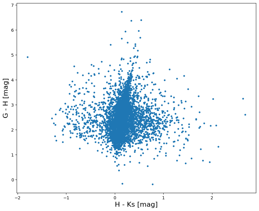
We now use the data we got from the cross-match to get a 2MASS/Gaia color-color diagram for all the sources in the low extinction sky regions covered by the MASH survey:

fig, ax = plt.subplots(figsize=(10, 8))
ax.plot(
    match_catalog["Hmag"] - match_catalog["Kmag"],
    match_catalog["Gmag"] - match_catalog["Hmag"],
    linestyle="",
    marker=".",
)
ax.set_xlabel("H - Ks [mag]", fontsize=16)
ax.set_ylabel("G - H [mag]", fontsize=16)
plt.show()