Multi-instrument, multi-wavelength study of high energy sources with the Virtual Observatory

François Bonnarel¹, Caroline Bot¹, Françoise Genova¹, René Goosmann¹, Manon Marchand¹, Ada Nebot¹.

1. Université de Strasbourg, CNRS, Observatoire Astronomique de Strasbourg, UMR 7550, F-67000, Strasbourg, France

This Notebook is based on the Euro-VO “Multi-instrument, multi-wavelength study of high energy sources with the Virtual Observatory” tutorial http://www.euro-vo.org/sites/default/files/documents/tutorial-highenergy_2016Nov.pdf.

Developed by Caroline Bot, François Bonnarel, René Goosmann and Françoise Genova. Adapted to a Jupyter Notebook by Ada Nebot.

---

Introduction

This tutorial demonstrates how to use several standard tools of the Virtual Observatory (VO) for data mining and multiple waveband data analysis. The step-by-step application below focuses on applications in the gamma-ray and high energy domain, but also involves observational data from other wavebands. The user may explore how to:

1. query astronomical catalogues in the gamma-ray and high energy spectral band using VO tools

2. cross-correlate catalogues to find an object at different photon energy bands

3. apply selection criteria when extracting sources from a catalogue

4. use the observational measures of the selected objects to explore possible correlations

5. visualize astronomical images from the radio up to the high energy domain

6. display spectral energy distributions obtained from different photometric data sets

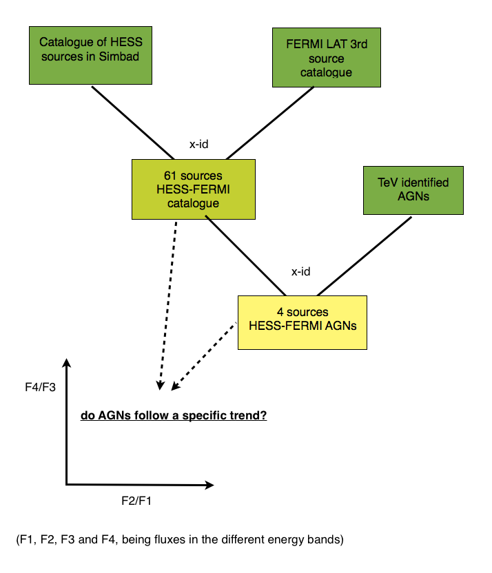
Schematic view of the scientific rationale of the tutorial:

# Standard Library
import pickle
from pathlib import Path

# Astronomy tools
from astropy import units as u
from astropy.coordinates import SkyCoord
from astropy.table import Table, hstack, join, unique, vstack

# Access astronomical databases
from astroquery.simbad import Simbad
from astroquery.vizier import Vizier

# Sky visualization
from ipyaladin import Aladin

# For plots
import plotly.express as px

Step #1 - Obtaining all HESS sources from SIMBAD

How to obtain a catalogue of all published HESS sources from the astronomical database SIMBAD.

The High Energy Stereoscopic System (HESS) is a Cherenkov telescope array detecting cosmic gamma-rays in the GeV—TeV range. Sources detected by HESS include supernova remnants (SNR), wind nebulae pulsars, active galactic nuclei (AGN) and others. The number of detected sources steadily grows and makes it possible to study certain sub-samples of the HESS catalogue. In the following, the HESS sources should be investigated with respect to their gamma-ray properties obtained from the second Fermi-LAT catalogue.

# Check which are the default fields
simbad = Simbad()
simbad.get_votable_fields()

['basic.main_id',
 'basic.ra',
 'basic.dec',
 'basic.coo_err_maj',
 'basic.coo_err_min',
 'basic.coo_err_angle',
 'basic.coo_wavelength',
 'basic.coo_bibcode']

# Check the available fields in a Simbad astroquery
simbad.list_votable_fields()

Table length=116

name	description	type
object	object	object
mesDiameter	Collection of stellar diameters.	table
mesPM	Collection of proper motions.	table
mesISO	Infrared Space Observatory (ISO) observing log.	table
mesSpT	Collection of spectral types.	table
allfluxes	all flux/magnitudes U,B,V,I,J,H,K,u_,g_,r_,i_,z_	table
ident	Identifiers of an astronomical object	table
flux	Magnitude/Flux information about an astronomical object	table
mesPLX	Collection of trigonometric parallaxes.	table
otypedef	all names and definitions for the object types	table
mesDistance	Collection of distances (pc, kpc or Mpc) by several means.	table
otypes	List of all object types associated with an object	table
mesVar	Collection of stellar variability types and periods.	table
mesXmm	XMM observing log.	table
...	...	...
R	Magnitude R	filter name
I	Magnitude I	filter name
J	Magnitude J	filter name
H	Magnitude H	filter name
K	Magnitude K	filter name
u	Magnitude SDSS u	filter name
g	Magnitude SDSS g	filter name
r	Magnitude SDSS r	filter name
i	Magnitude SDSS i	filter name
z	Magnitude SDSS z	filter name
G	Magnitude Gaia G	filter name
F150W	JWST NIRCam F150W	filter name
F200W	JWST NIRCam F200W	filter name
F444W	JWST NIRCan F444W	filter name

# Get more information about the field coordinatse
simbad.get_field_description("otype")

'Object type'

To check all available object types in Simbad go to http://simbad.u-strasbg.fr/simbad/sim-display?data=otypes

# Add the field otype and check that it is now included
simbad.add_votable_fields("otype")
# Check that it was added
simbad.get_votable_fields()

['basic.main_id',
 'basic.ra',
 'basic.dec',
 'basic.coo_err_maj',
 'basic.coo_err_min',
 'basic.coo_err_angle',
 'basic.coo_wavelength',
 'basic.coo_bibcode',
 'basic.otype']

# Query Simbad by catalog containing the keyword 'hess'
# and display the result
hess_simbad = simbad.query_catalog("HESS")
hess_simbad

Table length=114

main_id	ra	dec	coo_err_maj	coo_err_min	coo_err_angle	coo_wavelength	coo_bibcode	otype	catalog_id
	deg	deg	mas	mas	deg
object	float64	float64	float32	float32	int16	str1	object	object	object
HESS J0232+202	38.221666666666664	20.272499999999997	--	--	--		2007A&A...475L...9A	gam	HESS J0232+202
HESS J0534+220	83.5	22.0	--	--	--		2008ApJ...682L..41H	gam	HESS J0534+220
HESS J0535-691	83.97916666666666	-69.18611111111112	--	--	--		2019A&A...621A.138K	gam	HESS J0535-691
4FGL J0535.2-6736	84.00004166666666	-67.58541666666666	--	--	--	X	2012ApJ...759..123S	HXB	HESS J0536-675
HESS J0537-691	84.43333333333334	-69.16583333333334	--	--	--		2012A&A...545L...2H	gam	HESS J0537-691
HESS J0538-691	84.692	-69.103	--	--	--	G	2024ApJ...970L..21A	gam	HESS J0538-691
HD 259440	98.24690253194001	5.80032243218	0.0175	0.0163	90	O	2020yCat.1350....0G	HXB	HESS J0632+057
NAME MONOCEROS NEB	99.67916666666666	6.503333333333333	31000.0	18000.0	94		1988IRASP.C......0J	SNR	HESS J0632+058
NAME Vela X	128.287	-45.1901	--	--	--		2015ApJS..217....2M	Psr	HESS J0835-455
NAME Vela Jr SN	133.0	-46.333333333333336	--	--	--	R	2009BASI...37...45G	SNR	HESS J0852-463
HESS J1018-589	154.5	-58.9	--	--	--		2012Sci...335..189A	gam	HESS J1018-589
1FGL J1018.6-5856	154.73161487762	-58.94610423524998	0.0093	0.0094	90	O	2020yCat.1350....0G	HXB	HESS J1018-589A
PSR J1016-58	154.08860833333333	-58.953250000000004	1213.0	710.0	90	R	2015ApJ...814..128K	Psr	HESS J1018-589B
...	...	...	...	...	...	...	...	...	...
ARGO J1907+0627	287.051	6.3918800000000005	208416.0	208416.0	90	G	2020ApJ...905...76A	gam	HESS J1908+063
W 49b	287.7894	9.105899999999998	5000.0	5000.0	90	X	2022A&A...661A..38P	SNR	HESS J1911+090
ARGO J1912+1026	288.062	10.351599999999998	306640.0	306640.0	90	G	2020ApJ...905...76A	gam	HESS J1912+101
HESS J1915+115	288.75	11.500000000000002	--	--	--	G	2021ApJ...917....6A	gam	HESS J1915+115
HESS J1923+140	290.75	13.999999999999998	--	--	--	G	2021ApJ...917....6A	gam	HESS J1923+140
HESS J1923+141	290.75	14.1	--	--	--		2010ApJ...709L...6A	gam	HESS J1923+141
HAWC J1928+178	292.09999999999997	17.82	--	--	--	G	2021ApJ...917....6A	gam	HESS J1928+181
SNR G054.1+00.3	292.544	18.8394	314633.0	314633.0	90	G	2020ApJ...905...76A	SNR	HESS J1930+188
2MASS J19435624+2118233	295.98435	21.306494444444446	110.0	110.0	90	I	2003yCat.2246....0C	Bla	HESS J1943+213
HESS J1943+215	295.75	21.51833333333333	--	--	--		2012PASJ...64..100Y	gam	HESS J1943+215
QSO B2005-489	302.35579329135	-48.83159029195999	0.0258	0.0197	90	O	2020yCat.1350....0G	BLL	HESS J2009-488
QSO B2155-304	329.71693843745	-30.225588457719997	0.0171	0.0137	90	O	2020yCat.1350....0G	BLL	HESS J2158-302
QSO B2356-309	359.78293124841	-30.627964194039993	0.0937	0.0716	90	O	2020yCat.1350....0G	BLL	HESS J2359-306

f"There are {len(hess_simbad)} HESS sources in Simbad database."

'There are 114 HESS sources in Simbad database.'

Exercise: Do you know how to count how many HESS sources in Simbad are classified as HMXB? And as SNR? (answer in next cell, we use the pandas functionnalities)

df_hess_simbad = hess_simbad.to_pandas()
df_hess_simbad.groupby("otype").count()["main_id"]

otype
BLL     4
Bla     1
HXB     7
LXB     1
Psr    21
SNR    16
XB*     1
gam    62
reg     1
Name: main_id, dtype: int64

Step #2 - Projecting HESS sources onto the Fermi sky

Display the HESS sources in Galactic coordinates and overlay it on a view of an all-sky image survey conducted with Fermi LAT.

# Display the Fermi color HiPS
aladin = Aladin(survey="P/Fermi/color")
aladin

# Display the sources on top
aladin.add_table(hess_simbad, name="HESS-SIMBAD")

# Increase height of the widget
aladin.height = 600

** zoom out and move to see the points **

The HESS sources are overlayed on top of the Fermi images. If you don’t see them, zoom out and move around the sky to locate them around the Galactic Plane. By selecting a source you will see the main Simbad information of that source at the bottom of the AladinLite widget. You can change the image by selecting the stack layer.

# Select the "SNR" sources and overlay them
# Note that characters in python need that extra "b"
idx_SNR = hess_simbad["otype"] == ["SNR"]
aladin.add_table(hess_simbad[idx_SNR], name="SNR", color="red", shape="circle")

Scroll up to the widget to see the SNR in red.

Step #3 - Cross-identify HESS and Fermi LAT sources

Here we will cross-correlate the HESS source list with the complete set of objects appearing in the 3rd Fermi LAT catalogue.

Then we use the CDS XMatch service (http://cdsxmatch.u-strasbg.fr/) via the astroquery.XMatch.query module to look for spatial crossmatches

The cross-correlation will create a new, sub-catalogue of all HESS sources found in Simbad that also appear in the 3rd Fermi-LAT catalogue.

The Fermi Gamma Ray Space Telescope was launched in 2008 and observes astronomical objects across the 10 keV – 300 GeV band. The main instrument of the Fermi satellite is the Large Area Telescope (LAT), an imaging high-energy gamma-ray telescope covering the spectral range of 20 MeV – 300 GeV. The LAT has a very wide field of view, covering 20% of the sky at any time and scanning the complete sky every three hours. In the third Fermi-LAT catalogue (3FGL) all identified Fermi sources after 4 years of continuous survey were published together with basic measurements such as photometric fluxes in different spectral bands, an estimated gamma-ray spectral slope, or a variability flag.

In the following cross-identification process, it is assumed that the HESS source and its Fermi counterpart have an apparent angular distance of less then 1°, which is guided by the average angular resolution of the Fermi-LAT across the gamma-ray waveband. The angular resolution of the Fermi-LAT drops from 3° at 100 MeV to 0.04° at 100 GeV. Choosing a different limit for the angular distance thus favors associations with more objects at the low or at the high energy end of the Fermi-LAT band.

Find the VizieR name of the 3rd Fermi LAT catalogue.

catalog_list = Vizier.find_catalogs("Fermi LAT third catalog")
for k, v in catalog_list.items():
    print(k, ": ", v.description)

IX/67 :  Incremental Fermi LAT 4th source cat. (4FGL-DR3) (Fermi-LAT col., 2022)
J/ApJ/893/46 :  The fourth Fermi-GBM GRB catalog: 10 years (von Kienlin+, 2020)
J/ApJS/199/31 :  Fermi LAT second source catalog (2FGL) (Nolan+, 2012)
J/ApJS/218/23 :  Fermi LAT third source catalog (3FGL) (Acero+, 2015)
J/ApJS/223/28 :  The third Fermi/GBM GRB catalog (6yr) (Bhat+, 2016)
J/ApJS/247/33 :  The Fermi LAT fourth source catalog (4FGL) (Abdollahi+, 2020)
J/ApJS/263/24 :  The 4LAC-DR3 catalog (Ajello+, 2022)

Check the list of cadidate catalogs and select the one that interests us, i.e. “Fermi LAT third source catalog (3FGL) (Acero+, 2015)”. It’s identifier is: J/ApJS/218/23. VizieR might have several tables associated to this catalog. The next step is to see if the catalog has more than one table associated. We display table names and metadata:

# these two lines are commented out to prevent this pretty large catalog to be queried a lot of times.
# They should be executed the first time you do the tutorial to store the result in a pickle file.

vizier = Vizier(row_limit=-1)
catalog = vizier.get_catalogs("J/ApJS/218/23")

print(catalog)
print("Metadata of each table: ")
print(catalog[0].meta)

TableList with 3 tables:
	'0:J/ApJS/218/23/table4' with 19 column(s) and 4984 row(s) 
	'1:J/ApJS/218/23/table8' with 13 column(s) and 3034 row(s) 
	'2:J/ApJS/218/23/table3' with 2 column(s) and 12 row(s) 
Metadata of each table: 
{'ID': 'J_ApJS_218_23_table4', 'name': 'J/ApJS/218/23/table4', 'description': 'LAT 4-year catalog (3034 unique 3FGL sources)'}

There are three tables, each with a different number of columns and rows. To see what could be of interest, let’s display their description.

for i in range(len(catalog)):
    print(catalog[i].meta["name"], ": ", catalog[i].meta["description"])

J/ApJS/218/23/table4 :  LAT 4-year catalog (3034 unique 3FGL sources)
J/ApJS/218/23/table8 :  LAT 4-year catalog: spectral information
J/ApJS/218/23/table3 :  Definitions of the analysis flags

We can even visualise the first element of each table to have an idea of their content.

table0 = catalog[0]
table0[0]

Row index=0

3FGL	Na	RAJ2000	DEJ2000	amaj	amin	phi	Sig	F35	S25	Gamma	Mod	Var	Flag	Assoc	TeV	Class	ID	Simbad
		deg	deg	deg	deg	deg		1e-05 / (m2 s)	fW / m2
str13	int16	float32	float32	float32	float32	int16	float32	float32	float32	float32	str2	str1	str12	str18	str1	str5	str26	str6
J0000.1+6545	1	0.038	65.752	0.102	0.078	41	6.8	1.0	13.6	2.41	PL		3	2FGL J2359.6+6543c				Simbad

table1 = catalog[1]
table1[0]

Row index=0

File	3FGL	LC	F1	E_F1	F2	E_F2	F3	E_F3	F4	E_F4	F5	E_F5
			0.0001 / (m2 s)	0.0001 / (m2 s)	0.0001 / (m2 s)	0.0001 / (m2 s)	1e-05 / (m2 s)	1e-05 / (m2 s)	1e-06 / (m2 s)	1e-06 / (m2 s)	1e-06 / (m2 s)	1e-06 / (m2 s)
str13	str13	str2	float32	float32	float32	float32	float32	float32	float32	float32	float32	float32
J0000.1p6545	J0000.1+6545	LC	1.81	0.82	0.69	0.14	1.24	0.23	0.58	0.49	0.28	0.19

table2 = catalog[2]
table2[0]

Row index=0

Flag	Note
int16	str347
1	Source with TS>35, which went to TS<25 when changing the diffuse model (Section 3.7.3) or the analysis method (Section 3.7.4). Sources with TS<=35 are not flagged with this bit because normal statistical fluctuations can push them to TS<25.

J/ApJS/218/23/table4 and J/ApJS/218/23/table8 contain positional and spectral information respectively. The first table has several entries for the same source, so before performing the match, let’s restric the table to unique entries for the same source. We then match the tables based on the names in column 3FGL to get all information in a single table.

table0 = unique(table0, keys="3FGL")
FERMI = join(
    table0,
    table1,
    keys="3FGL",
    join_type="inner",
    metadata_conflicts="silent",
)
print("Number of matches :", len(FERMI))
FERMI[0]

Number of matches : 3034

Row index=0

3FGL	Na	RAJ2000	DEJ2000	amaj	amin	phi	Sig	F35	S25	Gamma	Mod	Var	Flag	Assoc	TeV	Class	ID	Simbad	File	LC	F1	E_F1	F2	E_F2	F3	E_F3	F4	E_F4	F5	E_F5
		deg	deg	deg	deg	deg		1e-05 / (m2 s)	fW / m2												0.0001 / (m2 s)	0.0001 / (m2 s)	0.0001 / (m2 s)	0.0001 / (m2 s)	1e-05 / (m2 s)	1e-05 / (m2 s)	1e-06 / (m2 s)	1e-06 / (m2 s)	1e-06 / (m2 s)	1e-06 / (m2 s)
str13	int16	float32	float32	float32	float32	int16	float32	float32	float32	float32	str2	str1	str12	str18	str1	str5	str26	str6	str13	str2	float32	float32	float32	float32	float32	float32	float32	float32	float32	float32
J0000.1+6545	1	0.038	65.752	0.102	0.078	41	6.8	1.0	13.6	2.41	PL		3	2FGL J2359.6+6543c				Simbad	J0000.1p6545	LC	1.81	0.82	0.69	0.14	1.24	0.23	0.58	0.49	0.28	0.19

We have a new table with 3034 FERMI sources with spatial and spectral information. We move on to cross-match this table with the HESS-Simbad sources. This time the match will be based on positions.

Lets have a look again a the hess_simbad table and it’s content.

hess_simbad[0:5]

Table length=5

main_id	ra	dec	coo_err_maj	coo_err_min	coo_err_angle	coo_wavelength	coo_bibcode	otype	catalog_id
	deg	deg	mas	mas	deg
object	float64	float64	float32	float32	int16	str1	object	object	object
HESS J0232+202	38.221666666666664	20.272499999999997	--	--	--		2007A&A...475L...9A	gam	HESS J0232+202
HESS J0534+220	83.5	22.0	--	--	--		2008ApJ...682L..41H	gam	HESS J0534+220
HESS J0535-691	83.97916666666666	-69.18611111111112	--	--	--		2019A&A...621A.138K	gam	HESS J0535-691
4FGL J0535.2-6736	84.00004166666666	-67.58541666666666	--	--	--	X	2012ApJ...759..123S	HXB	HESS J0536-675
HESS J0537-691	84.43333333333334	-69.16583333333334	--	--	--		2012A&A...545L...2H	gam	HESS J0537-691

# Create a skycoord object from the ra and dec columns
c_hess_simbad = SkyCoord(hess_simbad["ra"], hess_simbad["dec"])
c_fermi = SkyCoord(FERMI["RAJ2000"], FERMI["DEJ2000"])

# Set the maximum separation
max_sep = 1.0 * u.deg
# For each row in the first catalog, look for the closest neighbor
idx, d2d, d3d = c_hess_simbad.match_to_catalog_sky(c_fermi, 1)
sep_constraint = d2d < max_sep

# limit the tables to matches within the maximum separation
hess_simbad_matches = hess_simbad[sep_constraint]
fermi_matches = FERMI[idx[sep_constraint]]

# Look at the number of matches in each table within the maximum separation
print("Number of possible hess-simbad matches:", len(hess_simbad_matches))
print("Number of possible fermi matches:", len(fermi_matches))

Number of possible hess-simbad matches: 97
Number of possible fermi matches: 97

There are 83 HESS-Simbad-FERMI possible matches within 1 degree for each row in the first table! Tables hess_simbad_matches and fermi_matches are the matched sources in hess_simbad and fermi, respectively, which are separated by less than 1 deg. But ideally we would like to have the result as a single table including the angular separation between the matches. Let’s go do that.

# Add the separation to the fermi Table and concatenate the matched tables
fermi_matches["Ang_Sep"] = d2d[sep_constraint]
hess_simbad_fermi = hstack(
    [hess_simbad_matches, fermi_matches],
    metadata_conflicts="silent",
)

print("Number of possible HESS-Simbad-Fermi matches", len(hess_simbad_fermi))

Number of possible HESS-Simbad-Fermi matches 97

Note that the same Fermi source can be associated to different HESS sources. You can investigate those possible matches within 1deg (recommended) or limit to have unique entries. For the purpose of the exercice we choose option 2, but in general, we recommend to look at all possible matches to see which might be the true association (if any).

# Limit to unique 3FGL sources, this will keep the first row of each duplicate
# Note that one could sort them before that
hess_simbad_fermi.sort("Ang_Sep")
hess_simbad_fermi = unique(hess_simbad_fermi, keys="3FGL", keep="first")
hess_simbad_fermi

Table length=73

main_id	ra	dec	coo_err_maj	coo_err_min	coo_err_angle	coo_wavelength	coo_bibcode	otype	catalog_id	3FGL	Na	RAJ2000	DEJ2000	amaj	amin	phi	Sig	F35	S25	Gamma	Mod	Var	Flag	Assoc	TeV	Class	ID	Simbad	File	LC	F1	E_F1	F2	E_F2	F3	E_F3	F4	E_F4	F5	E_F5	Ang_Sep
	deg	deg	mas	mas	deg							deg	deg	deg	deg	deg		1e-05 / (m2 s)	fW / m2												0.0001 / (m2 s)	0.0001 / (m2 s)	0.0001 / (m2 s)	0.0001 / (m2 s)	1e-05 / (m2 s)	1e-05 / (m2 s)	1e-06 / (m2 s)	1e-06 / (m2 s)	1e-06 / (m2 s)	1e-06 / (m2 s)	deg
object	float64	float64	float32	float32	int16	str1	object	object	object	str13	int16	float32	float32	float32	float32	int16	float32	float32	float32	float32	str2	str1	str12	str18	str1	str5	str26	str6	str13	str2	float32	float32	float32	float32	float32	float32	float32	float32	float32	float32	float64
HESS J0232+202	38.221666666666664	20.272499999999997	--	--	--		2007A&A...475L...9A	gam	HESS J0232+202	J0232.8+2016	1	38.219	20.271	0.055	0.047	-4	7.2	0.4	4.9	2.03	PL				P	bll	1ES 0229+200	Simbad	J0232.8p2016	LC	0.23	0.29	0.18	0.05	0.25	0.11	0.46	0.31	0.42	0.22	0.0029157033593276618
HESS J0534+220	83.5	22.0	--	--	--		2008ApJ...682L..41H	gam	HESS J0534+220	J0534.5+2201	1	83.637	22.024	0.012	0.011	90	30.7	157.3	1471.9	2.23	EC	T		1FHL J0534.5+2201	P	PSR	PSR J0534+2200	Simbad	J0534.5p2201	LC	6.31	--	3.33	--	14.47	--	90.04	29.86	56.02	2.84	0.1292618808058602
HD 259440	98.24690253194001	5.80032243218	0.0175	0.0163	90	O	2020yCat.1350....0G	HXB	HESS J0632+057	J0633.7+0632	4	98.438	6.541	0.018	0.018	71	57.9	17.1	124.4	2.16	EC			2FGL J0633.7+0633		PSR	LAT PSR J0633+0632	Simbad	J0633.7p0632	LC	8.43	1.05	4.67	0.21	14.08	0.50	25.80	1.61	1.05	0.35	0.7646571241230222
NAME Vela X	128.287	-45.1901	--	--	--		2015ApJS..217....2M	Psr	HESS J0835-455	J0833.1-4511e	3	128.287	-45.190	--	--	--	--	18.3	244.8	2.41	PL		5	1FHL J0833.1-4511e	E	PWN	Vela X	Simbad	J0833.1-4511e	LC	37.18	--	8.19	--	14.46	--	31.87	--	6.87	--	0.00010275196628510123
NAME Vela Jr SN	133.0	-46.333333333333336	--	--	--	R	2009BASI...37...45G	SNR	HESS J0852-463	J0852.7-4631e	3	133.200	-46.520	--	--	--	30.3	13.0	147.1	1.94	PL	T	10	1FGL J0854.0-4632	E	SNR	Vela Jr	Simbad	J0852.7-4631e	LC	9.39	2.21	3.41	0.28	7.54	0.63	19.79	2.39	13.22	1.28	0.23205529470804162
PSR J1016-58	154.08860833333333	-58.953250000000004	1213.0	710.0	90	R	2015ApJ...814..128K	Psr	HESS J1018-589B	J1016.3-5858	2	154.079	-58.967	0.031	0.029	-86	18.9	7.8	65.5	2.35	EC		5	2FGL J1016.5-5858	E	PSR	PSR J1016-5857	Simbad	J1016.3-5858	LC	7.61	3.73	2.20	0.43	7.33	0.63	13.16	1.51	0.80	0.34	0.014613325460475186
1FGL J1018.6-5856	154.73161487762	-58.94610423524998	0.0093	0.0094	90	O	2020yCat.1350....0G	HXB	HESS J1018-589A	J1018.9-5856	4	154.730	-58.946	0.014	0.014	28	52.2	27.1	250.3	2.30	LP			1FHL J1018.9-5855	E	HMB	1FGL J1018.6-5856	Simbad	J1018.9-5856	LC	26.67	1.08	11.41	0.55	21.92	0.78	32.61	1.97	1.42	0.43	0.0008413415787775986
FGES J1023.3-5747	155.81326306	-57.77632889	--	--	--	G	2018A&A...612A...1H	gam	HESS J1023-575	J1023.1-5745	3	155.790	-57.759	0.018	0.018	-32	31.2	19.9	148.1	2.25	EC			1FGL J1023.0-5746	E	PSR	LAT PSR J1023-5746	Simbad	J1023.1-5745	LC	0.32	7.01	6.33	0.64	17.51	1.02	25.37	1.96	1.59	0.47	0.02131765846051888
PSR J1028-5819	157.11620000000002	-58.31837222222222	53.0	30.0	90	R	2015ApJ...814..128K	Psr	HESS J1026-582	J1028.4-5819	5	157.123	-58.320	0.012	0.012	-74	57.5	33.3	251.2	2.18	EC			1FHL J1028.4-5819		PSR	PSR J1028-5819	Simbad	J1028.4-5819	LC	13.98	3.65	9.39	0.68	26.78	0.91	50.11	2.32	3.55	0.60	0.0039260856722611575
Mrk 421	166.11380868146	38.20883291552	0.0124	0.0148	90	O	2020yCat.1350....0G	BLL	HESS J1104+382	J1104.4+3812	7	166.118	38.210	0.007	0.007	-12	190.3	30.3	383.0	1.77	PL	T		1FHL J1104.4+3812	P	BLL	Mkn 421	Simbad	J1104.4p3812	LC	10.19	0.30	4.80	0.09	17.98	0.39	82.34	2.40	42.61	1.71	0.0034909340127782604
PSR J1119-6127	169.80958333333334	-61.463750000000005	--	--	--		2000ApJ...541..367C	Psr	HESS J1119-614	J1119.1-6127	2	169.794	-61.466	0.029	0.027	-86	27.0	6.7	84.9	2.36	PL			2FGL J1118.8-6128	E	PSR	PSR J1119-6127	Simbad	J1119.1-6127	LC	7.39	1.66	2.72	0.22	5.57	0.43	10.59	1.24	1.39	0.40	0.007773186261269452
PSR J1301-6305	195.6999969482	-63.1800003052	--	--	--		2022ApJS..260...53A	Psr	HESS J1303-631	J1303.0-6312e	2	195.750	-63.200	--	--	--	7.6	1.6	22.7	1.64	PL			2FGL J1303.7-6316c	E	PWN	HESS J1303-631	Simbad	J1303.0-6312e	LC	0.00	1.01	0.47	0.30	0.97	0.50	2.67	1.40	3.50	0.70	0.03014314809054314
HESS J1357-645	209.25	-64.5	--	--	--			gam	HESS J1357-645	J1356.6-6428	2	209.164	-64.480	0.067	0.055	-75	17.9	2.6	41.8	2.56	PL			2FGL J1356.0-6436	E	PSR	PSR J1357-6429	Simbad	J1356.6-6428	LC	8.56	0.97	1.91	0.15	2.26	0.28	3.01	0.75	0.21	0.24	0.042089720952953324
...	...	...	...	...	...	...	...	...	...	...	...	...	...	...	...	...	...	...	...	...	...	...	...	...	...	...	...	...	...	...	...	...	...	...	...	...	...	...	...	...	...
HESS J1854+013	283.5	1.2999999999999998	--	--	--	G	2021ApJ...917....6A	gam	HESS J1854+013	J1855.9+0121e	6	283.990	1.355	--	--	--	68.3	70.7	535.7	2.20	LP	T		0FGL J1855.9+0126		SNR	W44	Simbad	J1855.9p0121e	LC	27.02	7.22	20.68	0.84	57.02	1.45	102.68	4.06	7.84	1.13	0.49293665293776606
HESS J1858+020	284.5833333333333	2.0900000000000003	--	--	--		2008A&A...477..353A	gam	HESS J1858+020	J1857.9+0210	2	284.490	2.170	0.060	0.058	13	15.2	8.2	68.0	2.36	LP		3,4	2FGL J1857.6+0211	E			Simbad	J1857.9p0210	LC	10.14	3.58	2.34	0.46	5.84	0.71	9.60	1.72	0.50	0.44	0.12288571482134578
HAWC J1907+085	286.79	8.57	--	--	--	G	2021ApJ...917....6A	gam	HESS J1907+089	J1904.9+0818	1	286.243	8.306	0.107	0.079	23	4.7	1.4	17.0	2.30	PL		4,5					Simbad	J1904.9p0818	LC	0.07	2.00	1.33	0.29	0.29	0.40	1.95	0.93	0.76	0.37	0.6020375632968096
ARGO J1907+0627	287.051	6.3918800000000005	208416.0	208416.0	90	G	2020ApJ...905...76A	gam	HESS J1908+063	J1907.9+0602	4	286.986	6.039	0.013	0.013	-46	84.0	38.4	319.1	2.24	EC			1FHL J1907.7+0600	E	PSR	LAT PSR J1907+0602	Simbad	J1907.9p0602	LC	30.88	1.76	12.22	0.32	31.16	0.80	60.89	2.65	3.08	0.62	0.35874848502120776
ARGO J1912+1026	288.062	10.351599999999998	306640.0	306640.0	90	G	2020ApJ...905...76A	gam	HESS J1912+101	J1908.9+1022	1	287.228	10.375	0.126	0.096	-82	6.4	1.7	27.2	2.59	PL		3,4					Simbad	J1908.9p1022	LC	3.88	1.57	1.05	0.24	1.57	0.43	1.10	0.88	0.37	0.30	0.8207313998263458
W 49b	287.7894	9.105899999999998	5000.0	5000.0	90	X	2022A&A...661A..38P	SNR	HESS J1911+090	J1910.9+0906	4	287.744	9.101	0.017	0.016	-80	41.8	20.3	183.5	2.18	LP			1FHL J1911.0+0905		snr	W 49B	Simbad	J1910.9p0906	LC	17.51	1.84	5.99	0.42	13.30	0.74	43.12	2.45	7.33	0.92	0.04510685664614893
HESS J1915+115	288.75	11.500000000000002	--	--	--	G	2021ApJ...917....6A	gam	HESS J1915+115	J1915.9+1112	2	289.000	11.216	0.147	0.120	2	10.7	3.8	38.2	2.41	LP		3,4	2FGL J1916.1+1106		spp		Simbad	J1915.9p1112	LC	6.28	1.22	1.81	0.27	3.05	0.58	4.21	1.42	0.00	0.34	0.3751428028503172
HESS J1923+141	290.75	14.1	--	--	--		2010ApJ...709L...6A	gam	HESS J1923+141	J1923.2+1408e	5	290.818	14.145	--	--	--	75.0	39.6	345.8	2.15	LP			0FGL J1923.0+1411	E	SNR	W51C	Simbad	J1923.2p1408e	LC	25.15	2.24	11.35	0.35	29.47	0.82	76.45	3.00	16.42	1.27	0.07983070024905738
SNR G054.1+00.3	292.544	18.8394	314633.0	314633.0	90	G	2020ApJ...905...76A	SNR	HESS J1930+188	J1928.4+1838	1	292.113	18.634	0.175	0.131	-23	5.8	1.6	21.9	2.42	PL		1,4,5					Simbad	J1928.4p1838	LC	0.27	1.95	0.99	0.26	1.26	0.39	1.65	0.93	0.64	0.37	0.45692117306583563
HAWC J1928+178	292.09999999999997	17.82	--	--	--	G	2021ApJ...917....6A	gam	HESS J1928+181	J1928.9+1739	3	292.237	17.657	0.080	0.058	-5	8.5	3.5	25.0	2.32	LP		3,4	2FGL J1928.8+1740c				Simbad	J1928.9p1739	LC	3.54	1.61	1.07	0.27	2.14	0.49	4.38	1.24	0.21	0.28	0.20879630393335458
QSO B2005-489	302.35579329135	-48.83159029195999	0.0258	0.0197	90	O	2020yCat.1350....0G	BLL	HESS J2009-488	J2009.3-4849	4	302.349	-48.828	0.018	0.018	-33	40.3	3.6	44.9	1.77	PL	T		1FHL J2009.4-4849	P	BLL	PKS 2005-489	Simbad	J2009.3-4849	LC	1.17	0.25	0.52	0.05	2.09	0.17	10.15	0.93	4.75	0.63	0.005735961234808655
QSO B2155-304	329.71693843745	-30.225588457719997	0.0171	0.0137	90	O	2020yCat.1350....0G	BLL	HESS J2158-302	J2158.8-3013	6	329.720	-30.227	0.009	0.009	-87	142.1	21.7	230.5	1.83	LP	T		1FHL J2158.8-3013	P	bll	PKS 2155-304	Simbad	J2158.8-3013	LC	6.47	0.45	3.62	0.09	13.42	0.36	57.34	2.10	23.98	1.35	0.00299836956521492
QSO B2356-309	359.78293124841	-30.627964194039993	0.0937	0.0716	90	O	2020yCat.1350....0G	BLL	HESS J2359-306	J2359.3-3038	3	359.829	-30.646	0.054	0.051	-7	11.1	0.6	6.6	2.02	PL			1FHL J2359.2-3037	P	bll	H 2356-309	Simbad	J2359.3-3038	LC	0.77	0.28	0.12	0.04	0.44	0.10	1.27	0.40	0.56	0.25	0.04355625621825019

f"There are {len(hess_simbad_fermi)} FERMI-HESS-Simbad matches"

'There are 73 FERMI-HESS-Simbad matches'

Some of these associations are of known nature.

Let’s query the ViZier catalog J/ApJ/810/14 : Third catalog of LAT-detected AGNs (3LAC) (Ackermann+, 2015). It lists 3LAC sources classified as AGNS. Let’s have a look at the catalog in question:

Vizier.ROW_LIMIT = -1
catalog = Vizier.get_catalogs("J/ApJ/810/14")
for tab in catalog:
    print(tab.meta["name"], ": ", tab.meta["description"])

J/ApJ/810/14/highlat :  High latitude (|b|>10deg) 3LAC full  sample and fluxes
J/ApJ/810/14/lowlat :  Low latitude (|b|<10deg) sample  and fluxes
J/ApJ/810/14/table7 :  Sources from earlier FGL catalogs missing in 3LAC
J/ApJ/810/14/table10 :  Properties of the 3FGL very-high-energy (VHE) AGNs
J/ApJ/810/14/table2 :  *List of ATCA blazar candidates

Table J/ApJ/810/14/table10 lists the properties of very-high-energy ANGs. Let’s have a look at that table:

table10 = catalog[3]
table10

Table length=55

3FGL	LL	VHE	SpCl	SEDCl	z	alpha	e_alpha	Var
str12	str1	str21	str6	str3	float32	float32	float32	float64
J0013.9-1853		SHBL J001355.9-185406	bll	HSP	0.094	1.935	0.167	36.46
J0033.6-1921		KUV 00311-1938	bll	HSP	0.610	1.715	0.035	64.62
J0035.9+5949	L	1ES J0033+595	bll	HSP	--	1.898	0.042	69.55
J0136.5+3905		RGB J0136+391	bll	HSP	--	1.696	0.025	62.30
J0152.6+0148		RGB J0152+017	bll	HSP	0.080	1.887	0.103	51.76
J0222.6+4301		3C 66A	bll	ISP	0.444	1.880	0.017	885.04
J0232.8+2016		1ES 0229+200	bll	HSP	0.139	2.025	0.150	49.16
J0303.4-2407		PKS 0301-243	bll	HSP	0.260	1.918	0.022	676.85
J0316.6+4119		IC 310	rdg	HSP	0.019	1.902	0.143	38.74
J0319.8+1847		RBS 0413	bll	HSP	0.190	1.572	0.102	76.33
J0319.8+4130		NGC 1275	rdg	ISP	0.018	1.985	0.014	622.21
J0349.2-1158		1ES 0347-121	bll	HSP	--	1.734	0.156	44.26
J0416.8+0104		1ES 0414+009	bll	HSP	0.287	1.745	0.114	55.85
...	...	...	...	...	...	...	...	...
J1517.6-2422		AP Lib	bll	LSP	0.048	2.112	0.026	60.31
J1555.7+1111		PG 1553+113	bll	HSP	--	1.604	0.025	123.55
J1653.9+3945		Markarian 501	bll	HSP	0.034	1.716	0.016	251.47
J1725.0+1152		1H 1720+117	bll	HSP	--	1.885	0.045	79.88
J1728.3+5013		1ES 1727+502	bll	HSP	0.055	1.960	0.065	54.08
J1743.9+1934		1ES 1741+196	bll	HSP	0.084	1.777	0.108	38.27
J2000.0+6509		1ES 1959+650	bll	HSP	0.047	1.883	0.022	158.37
J2001.1+4352	L	MAGIC J2001+435	bll	ISP	--	1.971	0.022	341.11
J2009.3-4849		PKS 2005-489	bll	-	0.071	1.773	0.031	131.06
J2158.8-3013		PKS 2155-304	bll	HSP	0.116	1.750	0.018	618.50
J2202.7+4217		BL Lacertae	bll	ISP	0.069	2.161	0.017	2340.22
J2250.1+3825		B3 2247+381	bll	HSP	0.119	1.912	0.074	52.42
J2347.0+5142	L	1ES 2344+514	bll	HSP	0.044	1.782	0.039	100.97
J2359.3-3038		H 2356-309	bll	HSP	0.165	2.022	0.115	40.97

There are no coordinates, only names are given in column _3FGL. Let’s see how many of these AGNs are within our table of matches hess_simbad_fermi:

hess_simbad_fermi_AGN = join(
    hess_simbad_fermi,
    table10,
    keys="3FGL",
    join_type="inner",
    metadata_conflicts="silent",
)
print("Number of matches :", len(hess_simbad_fermi_AGN))
hess_simbad_fermi_AGN

Number of matches : 5

Table length=5

main_id	ra	dec	coo_err_maj	coo_err_min	coo_err_angle	coo_wavelength	coo_bibcode	otype	catalog_id	3FGL	Na	RAJ2000	DEJ2000	amaj	amin	phi	Sig	F35	S25	Gamma	Mod	Var_1	Flag	Assoc	TeV	Class	ID	Simbad	File	LC	F1	E_F1	F2	E_F2	F3	E_F3	F4	E_F4	F5	E_F5	Ang_Sep	LL	VHE	SpCl	SEDCl	z	alpha	e_alpha	Var_2
	deg	deg	mas	mas	deg							deg	deg	deg	deg	deg		1e-05 / (m2 s)	fW / m2												0.0001 / (m2 s)	0.0001 / (m2 s)	0.0001 / (m2 s)	0.0001 / (m2 s)	1e-05 / (m2 s)	1e-05 / (m2 s)	1e-06 / (m2 s)	1e-06 / (m2 s)	1e-06 / (m2 s)	1e-06 / (m2 s)	deg
object	float64	float64	float32	float32	int16	str1	object	object	object	str13	int16	float32	float32	float32	float32	int16	float32	float32	float32	float32	str2	str1	str12	str18	str1	str5	str26	str6	str13	str2	float32	float32	float32	float32	float32	float32	float32	float32	float32	float32	float64	str1	str21	str6	str3	float32	float32	float32	float64
HESS J0232+202	38.221666666666664	20.272499999999997	--	--	--		2007A&A...475L...9A	gam	HESS J0232+202	J0232.8+2016	1	38.219	20.271	0.055	0.047	-4	7.2	0.4	4.9	2.03	PL				P	bll	1ES 0229+200	Simbad	J0232.8p2016	LC	0.23	0.29	0.18	0.05	0.25	0.11	0.46	0.31	0.42	0.22	0.0029157033593276618		1ES 0229+200	bll	HSP	0.139	2.025	0.150	49.16
Mrk 421	166.11380868146	38.20883291552	0.0124	0.0148	90	O	2020yCat.1350....0G	BLL	HESS J1104+382	J1104.4+3812	7	166.118	38.210	0.007	0.007	-12	190.3	30.3	383.0	1.77	PL	T		1FHL J1104.4+3812	P	BLL	Mkn 421	Simbad	J1104.4p3812	LC	10.19	0.30	4.80	0.09	17.98	0.39	82.34	2.40	42.61	1.71	0.0034909340127782604		Markarian 421	bll	HSP	0.031	1.772	0.008	755.10
QSO B2005-489	302.35579329135	-48.83159029195999	0.0258	0.0197	90	O	2020yCat.1350....0G	BLL	HESS J2009-488	J2009.3-4849	4	302.349	-48.828	0.018	0.018	-33	40.3	3.6	44.9	1.77	PL	T		1FHL J2009.4-4849	P	BLL	PKS 2005-489	Simbad	J2009.3-4849	LC	1.17	0.25	0.52	0.05	2.09	0.17	10.15	0.93	4.75	0.63	0.005735961234808655		PKS 2005-489	bll	-	0.071	1.773	0.031	131.06
QSO B2155-304	329.71693843745	-30.225588457719997	0.0171	0.0137	90	O	2020yCat.1350....0G	BLL	HESS J2158-302	J2158.8-3013	6	329.720	-30.227	0.009	0.009	-87	142.1	21.7	230.5	1.83	LP	T		1FHL J2158.8-3013	P	bll	PKS 2155-304	Simbad	J2158.8-3013	LC	6.47	0.45	3.62	0.09	13.42	0.36	57.34	2.10	23.98	1.35	0.00299836956521492		PKS 2155-304	bll	HSP	0.116	1.750	0.018	618.50
QSO B2356-309	359.78293124841	-30.627964194039993	0.0937	0.0716	90	O	2020yCat.1350....0G	BLL	HESS J2359-306	J2359.3-3038	3	359.829	-30.646	0.054	0.051	-7	11.1	0.6	6.6	2.02	PL			1FHL J2359.2-3037	P	bll	H 2356-309	Simbad	J2359.3-3038	LC	0.77	0.28	0.12	0.04	0.44	0.10	1.27	0.40	0.56	0.25	0.04355625621825019		H 2356-309	bll	HSP	0.165	2.022	0.115	40.97

There are a few AGNs ! Let’s have a look at their properties and see how they compare with the rest of the population.

Step #4 - Searchig for relative locations in a “high-energy color-color diagram”

How to trace various object properties of a given catalogue against each other and to point out specific sub-samples in the resulting plot.

The next goal is to look for correlations between different high-energy gamma-ray colors of the HESS sources that are also detected by Fermi. In stellar astronomy, tracing optical colors against each other gives a rather robust classification of different star types without having to do (more ambitious) spectroscopy. In the HESS-FERMI catalogue there is not much spectroscopic information available, but the different fluxes in F1—F5 coming from the 3FGL part can be used to eventually discriminate different sub-samples of the catalogue. Since a color is basically an observed flux ratio between two bands, constructing a color-color diagram has the great advantage to be independent of the distance to the objects.

The “color-color” diagram to be computed involves the following high-energy gamma-ray fluxes as measured by Fermi-LAT:

• F1: flux over 100 – 300 MeV

• F2: flux over 300 - 1000 MeV

• F3: flux over 1 - 3 GeV

• F4: flux over 3 - 10 GeV

• F5: flux over 10 - 100 GeV

Merge all the tables in one, but keeping their origin by adding a column with name Source. Add a column for the object type TYPE.

# Create a column with name Source to know  which will contain types as "All" for FERMI,
FERMI["Source"] = "FGL3"
hess_simbad_fermi["Source"] = "HESS-Simbad-3FGL"
hess_simbad_fermi_AGN["Source"] = "AGNs-3LAC"

# Create a column with name TYPE which will contain types as "All" for FERMI,
# Have to change to str since otype is of object type
FERMI["TYPE"] = "ALL"
hess_simbad_fermi["TYPE"] = hess_simbad_fermi["otype"].astype(str)
hess_simbad_fermi_AGN["TYPE"] = "AGN"

# Merge the tables vertically using vstack
Data = vstack(
    [FERMI, hess_simbad_fermi, hess_simbad_fermi_AGN],
    metadata_conflicts="silent",
)

# Create two new columns with the flux ratios
Data["F2_F1"] = Data["F2"] / Data["F1"]
Data["F4_F3"] = Data["F4"] / Data["F3"]

Save the file into for instance csv format and into a Panda kind of table to be able to use Plotly

# Write Table to csv format and to panda format
Data.write("Data" / Path("Data_FERMI-HESS-SIMBAD-AGN.csv"), overwrite=True)
Data = Data.to_pandas()

And now lets plot using Plotly:

• Flux ratios F2/F1 vs F4/F3

• In a log. scale

• Color coded according to the Source

• Using fancy markers

• Adding a legend

fig = px.scatter(
    Data,
    x="F2_F1",
    y="F4_F3",
    log_x=True,
    log_y=True,
    color="Source",
    hover_name="TYPE",
)
fig.update_traces(
    marker={"size": 12, "line": {"width": 2, "color": "DarkSlateGrey"}},
    selector={"mode": "markers"},
)
fig.show()

Note that when you move around with the mouse you get the values for each of the sources. You can activate or deactivate a type of Source in the plot by selecting it in the legend. You can zoom in and out, you can export as a png… and plenty more. Play a little bit with it.

Do the same as before but now color coded by object type.

# Plot same thing but color coded by the TYPE of object
fig = px.scatter(Data, "F2_F1", y="F4_F3", log_x=True, log_y=True, color="TYPE")
fig.update_traces(
    marker={"size": 12, "line": {"width": 2, "color": "DarkSlateGrey"}},
    selector={"mode": "markers"},
)
fig.show()

Step #5 – Display the location of interesting sources and search multi-wavelength data around them

How to obtain multi-wavelength images for the source you are interested in.

After isolating the 5 SIMBAD-confirmed BL Lac objects on the gamma-ray “color-color” diagram, this last step focuses on one particular object: PKS 2155-304, a peculiar BL Lac object known to be very variable on a wide spectral range and to show recurrent outbursts. A BL Lac object is a sub-type of active galactic nuclei, where the central engine around the accreting supermassive black hole launches magnetized, ballistic jets that reach out to kiloparsec scales while being nearly aligned with the line of sight of the observer. The emission from the jets is modeled as relativistically beamed synchrotron-self-Compton (SSC) emission produced in the hot plasma of the ejected jet material. The very hot electrons produce synchrotron emission that peaks in the radio band and then the very same electrons comptonize the synchrotron photons and up-scatter them to gamma-rays and beyond. However, in reality the question of the seed photons and the structure of the jet are still under investigation. A simple SSC interpretation of the broad band spectrum is challenged by the partially correlated variability seen between different spectral bands.

Broad-band spectrum reaching from the radio to the high-energy band (H.E.S.S., Fermi-LAT collaborations, ApJ 696, L150)

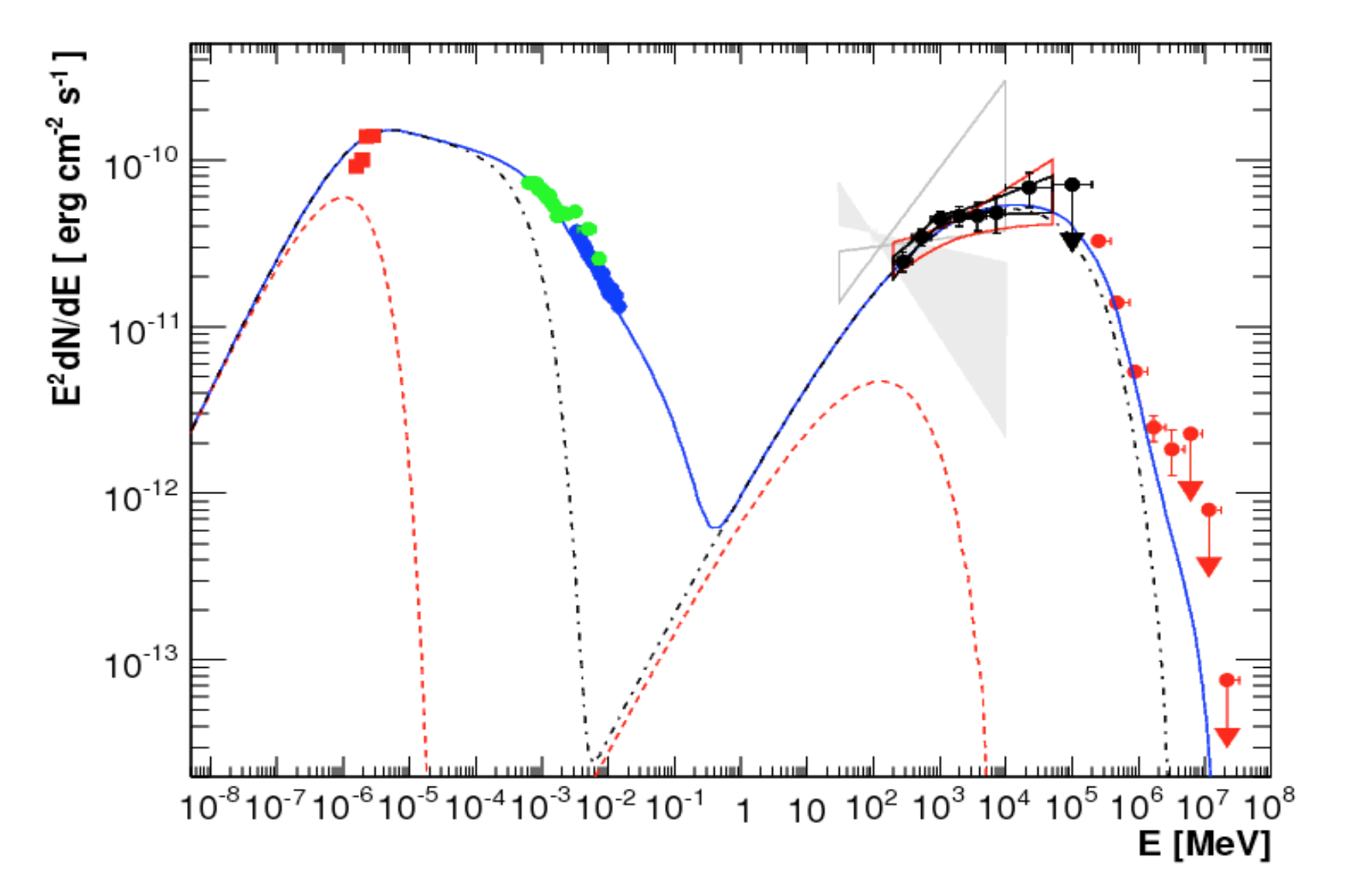
In the following, this tutorial shows how to obtain multi-waveband imaging for this source (PKS 2155-304).

Now, let’s plot again AladinLite with the catalog of AGNs on top on the Fermi image and centering around PKS 2155-30 and setting a field of view of 10 deg.

object_name = "PKS 2155-304"
aladin = Aladin(target=object_name, survey="P/Fermi/color", fov=10)
aladin

aladin.add_table(hess_simbad_fermi)
aladin.add_table(hess_simbad_fermi_AGN)

You can now see a marker on the source.

# object_coordinates = SkyCoord.from_name(object_name)
# here, were doing a query in a circle directly with an url to get the SED VizieR tool:
# query_url = f"https://vizier.cds.unistra.fr/viz-bin/sed?-c={object_coordinates.icrs.ra.deg},{object_coordinates.icrs.dec.deg}&-c.rs=5"
# since this can be a bit long, we saved the file in the folder Data. You can uncomment
# the url and comment the next line if you prefer to download the file:
query_url = "Data/sed_result.vot"
query = Table.read(query_url, format="votable")
query

Table length=1482

_RAJ2000	_DEJ2000	_tabname	_ID	_tab1_31	_tab1_32	sed_freq	sed_flux	sed_eflux	sed_filter
deg	deg			d	---	GHz	Jy	Jy	---
float64	float64	str32	str64	float64	float64	float64	float32	float32	str32
329.716940600	-30.225596400	I/297/out	NOMAD1===0597-1038713&-c=329.7169406 -30.2255964,eq=J2000&-c.rs=	--	0.0	181750	0.0524	--	2MASS:H
329.716940600	-30.225596400	I/297/out	NOMAD1===0597-1038713&-c=329.7169406 -30.2255964,eq=J2000&-c.rs=	--	0.0	241960	0.0435	--	2MASS:J
329.716983000	-30.225589000	I/305/out	GSC2.3===SCJS000019&-c=329.716983 -30.225589,eq=J2000&-c.rs=0.00	--	0.0	382540	0.0607	0.024	POSS-II:i
329.716983000	-30.225589000	I/305/out	GSC2.3===SCJS000019&-c=329.716983 -30.225589,eq=J2000&-c.rs=0.00	--	0.0	468430	0.0305	0.012	POSS-II:F
329.716983000	-30.225589000	I/305/out	GSC2.3===SCJS000019&-c=329.716983 -30.225589,eq=J2000&-c.rs=0.00	--	0.0	640580	0.0305	0.0088	POSS-II:J
329.716983000	-30.225589000	I/305/out	GSC2.3===SCJS000019&-c=329.716983 -30.225589,eq=J2000&-c.rs=0.00	--	0.0	674900	0.00193	0.00084	Johnson:B
329.716934920	-30.225604060	I/317/sample	PPMXL=1214064805186438959&-c=329.716935 -30.225604,eq=J2000&-c.r	--	0.0	138550	0.0597	0.0013	2MASS:Ks
329.716934920	-30.225604060	I/317/sample	PPMXL=1214064805186438959&-c=329.716935 -30.225604,eq=J2000&-c.r	--	0.0	181750	0.0524	0.0013	2MASS:H
329.716934920	-30.225604060	I/317/sample	PPMXL=1214064805186438959&-c=329.716935 -30.225604,eq=J2000&-c.r	--	0.0	241960	0.0435	0.0011	2MASS:J
329.716877000	-30.225596400	I/320/spm4	-c=329.7168770 -30.2255964,eq=J2000&-c.rs=0.004	--	--	138550	0.0597	--	2MASS:Ks
329.716877000	-30.225596400	I/320/spm4	-c=329.7168770 -30.2255964,eq=J2000&-c.rs=0.004	--	--	181750	0.0524	--	2MASS:H
329.716877000	-30.225596400	I/320/spm4	-c=329.7168770 -30.2255964,eq=J2000&-c.rs=0.004	--	--	241960	0.0435	--	2MASS:J
329.716877000	-30.225596400	I/320/spm4	-c=329.7168770 -30.2255964,eq=J2000&-c.rs=0.004	--	--	541430	0.00126	--	Johnson:V
...	...	...	...	...	...	...	...	...	...
329.716666700	-30.225555600	J/other/NewA/11.557/BLLac	recno=259	--	0.0	241960	0.0435	--	2MASS:J
329.716916700	-30.225583300	J/other/NewA/16.503/table1	recno=765	--	0.0	138550	0.0597	0.0013	2MASS:Ks
329.716916700	-30.225583300	J/other/NewA/16.503/table1	recno=765	--	0.0	181750	0.0524	0.0013	2MASS:H
329.716916700	-30.225583300	J/other/NewA/16.503/table1	recno=765	--	0.0	241960	0.0435	0.0011	2MASS:J
329.716938100	-30.225588300	J/other/AstBu/70.264/table	recno=784	--	0.0	4.8	0.492	0.061	:=4.8GHz
329.716958300	-30.225577800	J/other/RAA/24.E5011/catalog	recno=3243	--	0.0	13571	0.103	--	WISE:W4
329.716958300	-30.225577800	J/other/RAA/24.E5011/catalog	recno=3243	--	0.0	25934	0.0651	--	WISE:W3
329.716958300	-30.225577800	J/other/RAA/24.E5011/catalog	recno=3243	--	0.0	65172	0.0715	--	WISE:W2
329.716958300	-30.225577800	J/other/RAA/24.E5011/catalog	recno=3243	--	0.0	89490	0.0644	--	WISE:W1
329.716958300	-30.225577800	J/other/RAA/24.E5011/catalog	recno=3243	--	0.0	181750	0.0524	--	2MASS:H
329.716958300	-30.225577800	J/other/RAA/24.E5011/catalog	recno=3243	--	0.0	241960	0.0435	--	2MASS:J
329.716958300	-30.225577800	J/other/RAA/24.E5011/catalog	recno=3243	--	0.0	1.2967e+06	0.0124	--	GALEX:NUV
329.716958300	-30.225577800	J/other/RAA/24.E5011/catalog	recno=3243	--	0.0	1.9607e+06	0.00788	--	GALEX:FUV

query["nufnu"] = query["sed_freq"] * query["sed_flux"] * 1e-17
cc = 3e18
query["lambda"] = cc / query["sed_freq"] / 1e9
df_query = query.to_pandas()
fig = px.scatter(
    df_query,
    x="lambda",
    y="nufnu",
    log_x=True,
    log_y=True,
    color="_tabname",
)
fig.update_traces(
    marker={"size": 10, "line": {"width": 1, "color": "DarkSlateGrey"}},
    selector={"mode": "markers"},
)

fig.update_layout(
    xaxis_title="Wavelength [Å]",
    yaxis_title="vFv",
    title={
        "text": "Based on VizieR photometric Viewer",
        "y": 0.95,
        "x": 0.4,
        "xanchor": "center",
        "yanchor": "top",
    },
)

fig.show()