Coordinate conversion
In this example, we will load an archival all-sky Galactic reddening map, E(B-V), based on the derived reddening maps of Schlegel, Finkbeiner and Davis (1998). It has been translated into an HEALPix map in galactic coordinates by the Legacy Archive for Microwave Background Data Analysis LAMBDA. We’ll rotate it into equatorial coordinates for demonstration purpose.
Algorithm
It follows the following reasoning:
get the coordinates of the centers of the HEALPix map in galactic coordinates,
converts those to equatorial coordinates with the astropy library,
find the bilinear interpolation for the neighbors of each of these new coordinates using cdshealpix methods,
apply it to form a HEALPix map in the new coordinate system.
Disclaimer
This example was designed to illustrate the use of this library. This transformation is not the most precise you could get and should be used for visualizations or to have a quick view at maps in different coordinate systems. For scientific use, please have a look at the method rotate_alm in healpy or at the sht module of the ducc library that both implement the rotation in the spherical harmonics space.
[19]:
import cdshealpix

from mocpy import MOC, WCS
import astropy.units as u

from astropy.io import fits
from astropy.coordinates import SkyCoord, Angle

import matplotlib.pyplot as plt
import numpy as np
Fetching the HEALPix map from NASA archives
[20]:
ext_map = fits.open(
    "https://lambda.gsfc.nasa.gov/data/foregrounds/SFD/" + "lambda_sfd_ebv.fits"
)  # dowloading the map from the nasa archive
hdr = ext_map[0].header  # extracts the header
data_header = ext_map[1].header
data = ext_map[1].data  # extracts the data
ext_map.close()

hdr
[20]:
SIMPLE  =                    T / file does conform to FITS standard
BITPIX  =                   32 / number of bits per data pixel
NAXIS   =                    0 / number of data axes
EXTEND  =                    T / FITS dataset may contain extensions
COMMENT   FITS (Flexible Image Transport System) format is defined in 'Astronomy
COMMENT   and Astrophysics', volume 376, page 359; bibcode: 2001A&A...376..359H
DATE    = '2003-02-05T00:00:00' /file creation date (YYYY-MM-DDThh:mm:ss UT)
OBJECT  = 'ALL-SKY '           / Portion of sky given
COMMENT   This file contains an all-sky Galactic reddening map, E(B-V), based on
COMMENT   the derived reddening maps of Schlegel, Finkbeiner and Davis (1998).
COMMENT   Software and data files downloaded from their website were used to
COMMENT   interpolate their high resolution dust maps onto pixel centers
COMMENT   appropriate for a HEALPix Nside=512 projection in Galactic
COMMENT   coordinates. This file is distributed and maintained by LAMBDA.
REFERENC= 'Legacy Archive for Microwave Background Data Analysis (LAMBDA)      '
REFERENC= '                http://lambda.gsfc.nasa.gov/                        '
REFERENC= 'Maps of Dust Infrared Emission for Use in Estimation of Reddening an'
REFERENC= ' Cosmic Microwave Background Radiation Foregrounds',                '
REFERENC= ' Schlegel, Finkbeiner & Davis 1998 ApJ 500, 525                     '
REFERENC= 'Berkeley mirror site for SFD98 data: http://astron.berkeley.edu/dust'
REFERENC= 'Princeton mirror site for SFD98 data:                               '
REFERENC= '                           http://astro/princeton.edu/~schlegel/dust'
REFERENC= 'HEALPix Home Page: http://www.eso.org/science/healpix/              '
RESOLUTN=                    9 / Resolution index
SKYCOORD= 'Galactic'           / Coordinate system
PIXTYPE = 'HEALPIX '           / Pixel algorithm
ORDERING= 'NESTED  '           / Ordering scheme
NSIDE   =                  512 / Resolution parameter
NPIX    =              3145728 / # of pixels
FIRSTPIX=                    0 / First pixel (0 based)
LASTPIX =              3145727 / Last pixel (0 based)
Let’s also have a look at the data header
[21]:
data_header
[21]:
XTENSION= 'BINTABLE'           /binary table extension
BITPIX  =                    8 /8-bit bytes
NAXIS   =                    2 /2-dimensional binary table
NAXIS1  =                    8 /width of table in bytes
NAXIS2  =              3145728 /number of rows in table
PCOUNT  =                    0 /size of special data area
GCOUNT  =                    1 /one data group (required keyword)
TFIELDS =                    2 /number of fields in each row
COMMENT
COMMENT  *** End of mandatory fields ***
COMMENT
COMMENT
COMMENT  *** Column names ***
COMMENT
TTYPE1  = 'TEMPERATURE'        /label for field   1
COMMENT
COMMENT  *** Column formats ***
COMMENT
TFORM1  = 'E       '           /data format of field: 4-byte REAL
TUNIT1  = 'magnitudes'         /physical unit of field
TTYPE2  = 'N_OBS   '           /label for field   2
TFORM2  = 'E       '           /data format of field: 4-byte REAL
TUNIT2  = 'counts  '           /physical unit of field
EXTNAME = 'Archive Map Table'  /name of this binary table extension
DATE    = '2003-02-05T00:00:00' /Table creation date
PIXTYPE = 'HEALPIX '           /Pixel algorithm
ORDERING= 'NESTED  '           /Ordering scheme
NSIDE   =                  512 /Resolution parameter
FIRSTPIX=                    0 /First pixel (0 based)
LASTPIX =              3145727 /Last pixel (0 based)
COMMENT   The TEMPERATURE field contains E(B-V) in magnitudes.
COMMENT   N_obs is set to 1 for all pixels. The N_obs field is filled
COMMENT    only to provide a format consistent with that used by
COMMENT    WMAP products.
After learning that the magnitudes are stored in 'TEMPERATURE', we can extract all useful information.
[22]:
extinction_values = data["TEMPERATURE"]
nside = hdr["NSIDE"]
norder = hdr["RESOLUTN"]
Coordinate conversion
We first create an HEALPix grid at order 9 (like the original) in nested ordering
[23]:
healpix_index = np.arange(12 * 4**norder, dtype=np.uint64)
print(
    f"We can check that the NPIX value corresponds to the one in the header here: {len(healpix_index)}"
)
We can check that the NPIX value corresponds to the one in the header here: 3145728
Then, we get the coordinates of the centers of these healpix cells
[24]:
center_coordinates_in_equatorial = cdshealpix.healpix_to_skycoord(
    healpix_index, depth=norder
)  # this function works for nested maps, see cdshealpix documentation
center_coordinates_in_equatorial
[24]:
<SkyCoord (ICRS): (ra, dec) in deg
    [( 45.        ,  0.0746039 ), ( 45.08789062,  0.14920793),
     ( 44.91210938,  0.14920793), ..., (315.08789062, -0.14920793),
     (314.91210938, -0.14920793), (315.        , -0.0746039 )]>
Conversion into galactic coordinates with astropy method
[25]:
center_coordinates_in_galactic = center_coordinates_in_equatorial.galactic
center_coordinates_in_galactic
[25]:
<SkyCoord (Galactic): (l, b) in deg
    [(176.8796283 , -48.85086427), (176.89078038, -48.7358142 ),
     (176.70525363, -48.86216423), ..., ( 48.82487228, -28.4122831 ),
     ( 48.7216889 , -28.26178141), ( 48.84578935, -28.29847774)]>
Calculate the bilinear interpolation that must be applied to each HEALPix cell to obtain the magnitude values in the other coordinate system.
[26]:
healpix, weights = cdshealpix.bilinear_interpolation(
    center_coordinates_in_galactic.l, center_coordinates_in_galactic.b, depth=norder
)
# then apply the interpolation
ext_map_equatorial_nested = (extinction_values[healpix.data] * weights.data).sum(axis=1)
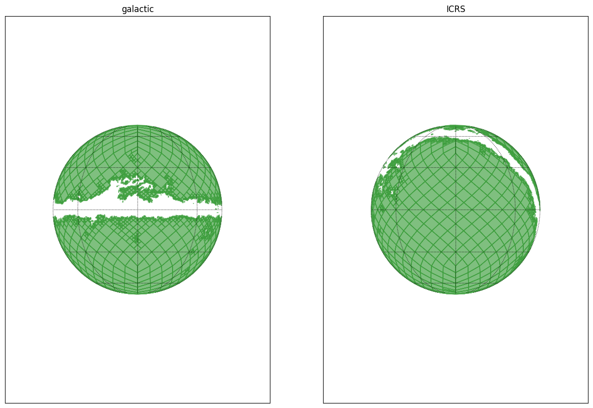
Convert the two HEALPix into MOCs for visualization
We produce the extinction MOCs by excluding the high extinction regions. This allows to have a clear view of the position of the galactic disc.
[27]:
# For the HEALPix in equatorial coordinate system
low_extinction_index_equatorial = np.where(ext_map_equatorial_nested < 0.5)[0]
moc_low_extinction_equatorial = MOC.from_healpix_cells(
    ipix=low_extinction_index_equatorial,
    depth=np.full((len(low_extinction_index_equatorial)), norder),
    max_depth=norder,
)

# For the HEALPix in galactic coordinate system
low_extinction_index_galactic = np.where(extinction_values < 0.5)[0]
moc_low_extinction_galactic = MOC.from_healpix_cells(
    ipix=low_extinction_index_galactic,
    depth=np.full((len(low_extinction_index_galactic)), norder),
    max_depth=norder,
)

# Plot the MOCs using matplotlib
fig = plt.figure(figsize=(15, 10))
# Define a astropy WCS from the mocpy.WCS class
with WCS(
    fig,
    fov=120 * u.deg,
    center=SkyCoord(0, 0, unit="deg", frame="icrs"),
    coordsys="icrs",
    rotation=Angle(0, u.degree),
    projection="SIN",
) as wcs:
    ax1 = fig.add_subplot(121, projection=wcs, aspect="equal", adjustable="datalim")
    ax2 = fig.add_subplot(122, projection=wcs, aspect="equal", adjustable="datalim")
    moc_low_extinction_galactic.fill(
        ax=ax1, wcs=wcs, alpha=0.5, fill=True, color="green"
    )
    moc_low_extinction_equatorial.fill(
        ax=ax2, wcs=wcs, alpha=0.5, fill=True, color="green"
    )

ax1.set(xlabel="l", ylabel="b", title="galactic")
ax2.set(xlabel="ra", ylabel="dec", title="ICRS")

ax1.grid(color="black", linestyle="dotted")
ax2.grid(color="black", linestyle="dotted")
plt.show()